Spatial Interaction Analysis#
Understanding how different cell types and signaling molecules are spatially organized within tissues is fundamental to deciphering the mechanisms of cell-cell communication and tissue function. This notebook demonstrates spatial interaction analysis using the exprmat package, covering both density-based and graph-based approaches. We construct expression density maps from spatial imaging data to visualize the spatial distribution of specific markers and cell types, compute density intersections to identify colocalization hotspots, and perform permutation-based spatial ligand-receptor interaction testing. The notebook also demonstrates CellNEST analysis for inferring cell-cell communication networks from spatial transcriptomics data, identifying ligand-receptor pairs and signaling relays that mediate intercellular interactions within the tissue microenvironment.
[1]:
%load_ext autoreload
%autoreload 2
[2]:
import exprmat as em
em.setwd('../../../data')
ver = em.version()
[i] exprmat 0.2.66 / exprmat-db 0.2.66
[i] os: posix (linux)  platform version: 6.8.0-90-generic
[i] loaded configuration from /home/data/yangz/.exprmatrc
[i] current working directory: /home/data/yangz/packages/exprmat/data
[i] current database directory: /home/data/yangz/packages/database (0.2.66)
[i] resident memory: 776.18 MiB
[i] virtual memory: 5.95 GiB
[3]:
expm = em.load_experiment('expm/codex')
━━━━━━━━━━━━━━━━━━━━━━━━━━ loading samples 2 / 2 (00:01 < 00:00)
[!] integrated mudata object is not generated.
Density based interaction#
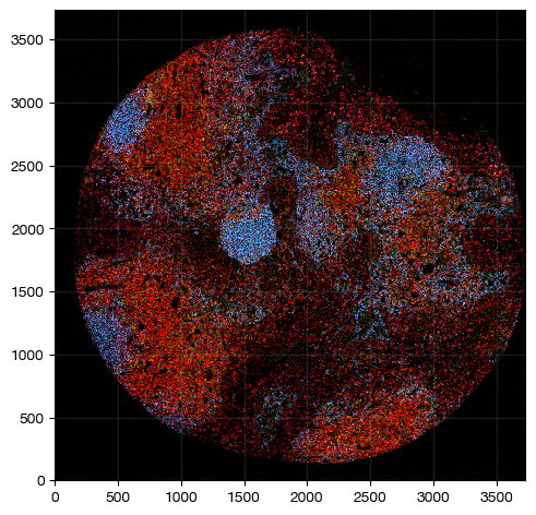
For dataset with low spatial resolution, expression densities may become a smoothed imputed intensity for interaction partners, and can be easily expanded and diffused to support diffusion ranges.
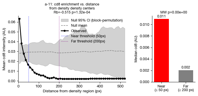
For high-resolution data but without segmentation masks of good quality, the operations on expression densities will preserve the logical selection of target cell pixels and perform distance analysis. Cell density can provide information on correlations of cell occurance
[4]:
expm.spatial_cell.summary(run_on_samples = ['a-11'])
a-11
├── adjusted  of shape 3733 ✗ 3732 ✗ 6
│       [0] cd4   [1] cd8   [2] dapi  [3] cd45  [4] cd20  [5] cd31
├── flow  of shape 3733 ✗ 3732 ✗ 4
│       [0] r            [1] g            [2] b            [3] probability
├── mask  of shape 3733 ✗ 3732
├── mixed-membrane  of shape 3733 ✗ 3732 ✗ 1
│       [0] mixed
├── origin  of shape 3733 ✗ 3732 ✗ 59
│       [ 0] dapi        [ 1] cd45        [ 2] cd11c       [ 3] bcl2        [ 4] cd90
│       [ 5] foxp3       [ 6] egfr        [ 7] p16         [ 8] pd1         [ 9] cd206
│       [10] cd45ro      [11] il10        [12] cd56        [13] cd11b       [14] cd31
│       [15] cd163       [16] cd21        [17] cd8         [18] pnad        [19] cd20
│       [20] cxcr5       [21] ki67        [22] lag3        [23] cd73        [24] cd16
│       [25] asma        [26] icos        [27] cd25        [28] coliv       [29] pdgfrb
│       [30] cd4         [31] cd68        [32] cd34        [33] vimentin    [34] podoplanin
│       [35] hladr       [36] cxcl12      [37] cd3         [38] fap         [39] cd138
│       [40] tbet        [41] periostin   [42] spp1        [43] s100a8a9    [44] clec9a
│       [45] cd45ra      [46] caix        [47] gzmb        [48] bcat        [49] sox2
│       [50] pdl1        [51] mmp9        [52] tcrgd       [53] cd38        [54] cd69
│       [55] cd15        [56] ido1        [57] mct1        [58] panck
└── segmentation-rgb  of shape 3733 ✗ 3732 ✗ 3
        [0] r  [1] g  [2] b
[5]:
expm.spatial_cell.image_auto_histogram(
    run_on_samples = True,
    channels = [
        'origin/cd4', 'origin/cd8', 'origin/dapi', 'origin/cd45',
        'origin/cd20', 'origin/cd31', 'origin/foxp3'
    ],
    key_added = 'adjusted',
    low_pct = 0.5,
    high_pct = 99.5
)
[7]:
fig = expm.spatial_cell.plot_spatial(
    run_on_samples = ['a-11'],
    channels = ['adjusted/cd4', 'adjusted/foxp3', 'adjusted/cd20'],
    channel_colors = ['red', 'green', "#4c85ff"],
    channel_intensities = [1, 1, 1],
    plot_embeddings = { 'visible': False, },
    figsize = (5, 5),
    ticks = True
)
[8]:
expm.spatial_cell.density_image(
    run_on_samples = ['a-11'],
    source_channel = ['adjusted/cd8', 'adjusted/cd4', 'adjusted/cd20', 'adjusted/foxp3'],
    target_image = 'density',
    target_channel = None,
    downresolution = 16
)
[9]:
expm.spatial_cell.summary(
    run_on_samples = ['a-11'],
)
a-11
├── adjusted  of shape 3733 ✗ 3732 ✗ 7
│       [0] cd4    [1] cd8    [2] dapi   [3] cd45   [4] cd20   [5] cd31   [6] foxp3
├── flow  of shape 3733 ✗ 3732 ✗ 4
│       [0] r            [1] g            [2] b            [3] probability
├── mask  of shape 3733 ✗ 3732
├── mixed-membrane  of shape 3733 ✗ 3732 ✗ 1
│       [0] mixed
├── origin  of shape 3733 ✗ 3732 ✗ 59
│       [ 0] dapi        [ 1] cd45        [ 2] cd11c       [ 3] bcl2        [ 4] cd90
│       [ 5] foxp3       [ 6] egfr        [ 7] p16         [ 8] pd1         [ 9] cd206
│       [10] cd45ro      [11] il10        [12] cd56        [13] cd11b       [14] cd31
│       [15] cd163       [16] cd21        [17] cd8         [18] pnad        [19] cd20
│       [20] cxcr5       [21] ki67        [22] lag3        [23] cd73        [24] cd16
│       [25] asma        [26] icos        [27] cd25        [28] coliv       [29] pdgfrb
│       [30] cd4         [31] cd68        [32] cd34        [33] vimentin    [34] podoplanin
│       [35] hladr       [36] cxcl12      [37] cd3         [38] fap         [39] cd138
│       [40] tbet        [41] periostin   [42] spp1        [43] s100a8a9    [44] clec9a
│       [45] cd45ra      [46] caix        [47] gzmb        [48] bcat        [49] sox2
│       [50] pdl1        [51] mmp9        [52] tcrgd       [53] cd38        [54] cd69
│       [55] cd15        [56] ido1        [57] mct1        [58] panck
├── segmentation-rgb  of shape 3733 ✗ 3732 ✗ 3
│       [0] r  [1] g  [2] b
└── density  of shape 233 ✗ 233 ✗ 4
        [0] cd8    [1] cd4    [2] cd20   [3] foxp3
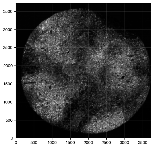
For example, the combinated density of CD4+ FOXP3+ regulatory T cells can be masked as follows:
[11]:
expm.spatial_cell.density_intersection(
    run_on_samples = ['a-11'],
    source_densities = ['density/cd4', 'density/foxp3'],
    diffusion = 2,
    target_image = 'treg',
    target_channel = 'density'
)
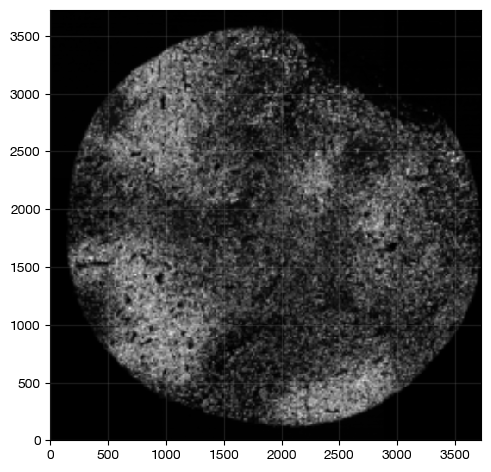
This is the double-positive density mask, compared to the CD4 single mask
[12]:
fig = expm.spatial_cell.plot_spatial(
    run_on_samples = ['a-11'],
    channels = ['treg/density'],
    channel_colors = ["white"],
    channel_intensities = [1],
    plot_embeddings = { 'visible': False, },
    figsize = (5, 5),
    ticks = True
)
[13]:
fig = expm.spatial_cell.plot_spatial(
    run_on_samples = ['a-11'],
    channels = ['density/cd4'],
    channel_colors = ["white"],
    channel_intensities = [1],
    plot_embeddings = { 'visible': False, },
    figsize = (5, 5),
    ticks = True
)
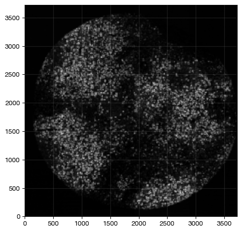
Or we may further watch for the colocalization area between Tregs and CD8+ T cells
[18]:
expm.spatial_cell.density_intersection(
    run_on_samples = ['a-11'],
    source_densities = ['density/cd4', 'density/foxp3', 'density/cd8'],
    diffusion = 0,
    target_image = 'treg-t8',
    target_channel = 'density'
)
[19]:
fig = expm.spatial_cell.plot_spatial(
    run_on_samples = ['a-11'],
    channels = ['treg-t8/density'],
    channel_colors = ["white"],
    channel_intensities = [1],
    plot_embeddings = { 'visible': False, },
    figsize = (5, 5),
    ticks = True
)
Initialize density maps from cell density#
Density maps can also be kernel density estimates from scatters
[32]:
expm.spatial_cell['a-11'].obs[['x', 'y', 'leiden', 'cell.type']]
[32]:
| x | y | leiden | cell.type | |
|---|---|---|---|---|
| a-11:c1 | 2100.405405 | 123.478764 | 18 | Unk |
| a-11:c2 | 2130.552743 | 123.552743 | 5 | B |
| a-11:c3 | 2149.627451 | 125.058824 | 18 | Unk |
| a-11:c4 | 1553.190476 | 123.396825 | 13 | Unk |
| a-11:c5 | 2209.738532 | 125.977064 | 5 | gdT |
| ... | ... | ... | ... | ... |
| a-11:c48512 | 1731.616099 | 3574.241486 | 13 | gdT |
| a-11:c48513 | 1774.181435 | 3574.426160 | 13 | T4 |
| a-11:c48514 | 1699.267399 | 3576.263736 | 11 | Epi |
| a-11:c48515 | 1754.540179 | 3575.816964 | 9 | Unk |
| a-11:c48516 | 1829.691120 | 3576.455598 | 13 | gdT |
47396 rows × 4 columns
[33]:
expm.spatial_cell.density_from_spots(
    run_on_samples = ['a-11'],
    category = 'cell.type',
    source_channel = 'origin/dapi',
    target_image = 'ctdens',
    downresolution = 16,
)
[34]:
expm.spatial_cell.summary(
    run_on_samples = ['a-11'],
)
a-11
├── adjusted  of shape 3733 ✗ 3732 ✗ 7
│       [0] cd4    [1] cd8    [2] dapi   [3] cd45   [4] cd20   [5] cd31   [6] foxp3
├── flow  of shape 3733 ✗ 3732 ✗ 4
│       [0] r            [1] g            [2] b            [3] probability
├── mask  of shape 3733 ✗ 3732
├── mixed-membrane  of shape 3733 ✗ 3732 ✗ 1
│       [0] mixed
├── origin  of shape 3733 ✗ 3732 ✗ 59
│       [ 0] dapi        [ 1] cd45        [ 2] cd11c       [ 3] bcl2        [ 4] cd90
│       [ 5] foxp3       [ 6] egfr        [ 7] p16         [ 8] pd1         [ 9] cd206
│       [10] cd45ro      [11] il10        [12] cd56        [13] cd11b       [14] cd31
│       [15] cd163       [16] cd21        [17] cd8         [18] pnad        [19] cd20
│       [20] cxcr5       [21] ki67        [22] lag3        [23] cd73        [24] cd16
│       [25] asma        [26] icos        [27] cd25        [28] coliv       [29] pdgfrb
│       [30] cd4         [31] cd68        [32] cd34        [33] vimentin    [34] podoplanin
│       [35] hladr       [36] cxcl12      [37] cd3         [38] fap         [39] cd138
│       [40] tbet        [41] periostin   [42] spp1        [43] s100a8a9    [44] clec9a
│       [45] cd45ra      [46] caix        [47] gzmb        [48] bcat        [49] sox2
│       [50] pdl1        [51] mmp9        [52] tcrgd       [53] cd38        [54] cd69
│       [55] cd15        [56] ido1        [57] mct1        [58] panck
├── segmentation-rgb  of shape 3733 ✗ 3732 ✗ 3
│       [0] r  [1] g  [2] b
├── density  of shape 233 ✗ 233 ✗ 4
│       [0] cd8    [1] cd4    [2] cd20   [3] foxp3
├── treg  of shape 3728 ✗ 3728 ✗ 1
│       [0] density
├── treg-t8  of shape 3728 ✗ 3728 ✗ 1
│       [0] density
└── ctdens  of shape 233 ✗ 233 ✗ 11
        [ 0] b     [ 1] ec    [ 2] epi   [ 3] fib   [ 4] mye   [ 5] nk    [ 6] t4    [ 7] t8
        [ 8] treg  [ 9] unk   [10] gdt
[36]:
fig = expm.spatial_cell.plot_spatial(
    run_on_samples = ['a-11'],
    channels = ['ctdens/t8'],
    channel_colors = ["white"],
    channel_intensities = [1],
    plot_embeddings = { 'visible': False, },
    figsize = (5, 5),
    ticks = True
)
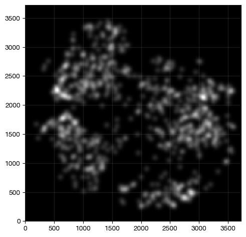
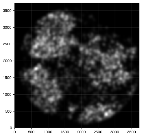
Gene expression densities can also be derived
[6]:
expm.spatial_cell.density_from_expression(
    run_on_samples = ['a-11'],
    feature = 'CD8',
    layer = 'compensated',
    source_channel = 'origin/dapi',
    target_image = 'expression',
    downresolution = 16,
)
[9]:
fig = expm.spatial_cell.plot_spatial(
    run_on_samples = ['a-11'],
    channels = ['expression/cd8'],
    channel_colors = ["white"],
    channel_intensities = [1],
    plot_embeddings = { 'visible': False, },
    figsize = (5, 5),
    ticks = True
)
Downstream analysis of density maps#
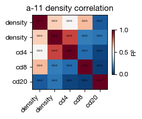
Density maps can be useful as a proxy of smoothed gene expression in spatial context.
[25]:
fig = expm.spatial_cell.plot_density_correlation(
    run_on_samples = ['a-11'],
    x_channels = ['treg-t8/density', 'treg/density', 'density/cd4', 'density/cd8', 'density/cd20'],
    y_channels = ['treg-t8/density', 'treg/density', 'density/cd4', 'density/cd8', 'density/cd20'],
    cmap = 'rdbu/r',
    figsize = (3, 2.5),
    dpi = 100,
)
[28]:
fig = expm.spatial_cell.plot_density_cooccurance(
    run_on_samples = ['a-11'],
    x_channel = 'treg/density',
    y_channel = 'density/cd8',
    x_threshold = 0.8,
    n_permutations = 100,
    max_distance = None,
    near_threshold = 50,
    far_threshold = 200,
    n_distance_bins = 50,
    random_state = 42,
    figsize = (8, 3),
)
Spatial Ligand-receptor Permutation Test#
CellChat’s permutation test variation is implemented for spatial data.
[6]:
expm = em.load_experiment('expm/visium')
━━━━━━━━━━━━━━━━━━━━━━━━━━ loading samples 8 / 8 (00:03 < 00:00)
[5]:
sample = 'p2-t5'
[16]:
expm.spatial_bin.view(sample)
annotated data of size 1470 × 35554
    obs : sample <cat> <c/sample> batch <cat> <c/batch> group <cat> <c> modality <cat> <c/modality>
          taxa <cat> <c/taxa> barcode <o> <o> ubc <o> <o> in.tissue <i64> <bool/intissue>
          row <i64> <f/coordinate/row> col <i64> <f/coordinate/col> y <i64> <f/coordinate/y>
          x <i64> <f/coordinate/x> leiden <cat> <c> spagcn.domain <cat> <c/domain>
          spagcn.refined <cat> <c/domain> imagerow <f64> imagecol <f64>
          deepst.domain <cat> <c/domain> deepst.refined <cat> <c/domain> integrated <cat>
          metagene.17 <f64> <f> ep1 <f32> ep2 <f32>
    var : chr <cat> <c/chromosome> start <i64> <i> end <i64> <i> strand <cat> <c/strand> id <o> <o>
          subtype <cat> <c/gsubtype> gene <cat> <o/gene> tlen <f64> <i/tlen> cdslen <i64> <i/cdslen>
          assembly <cat> <c> uid <o> <o/ugene> vst.means <f64> <f> vst.vars <f64> <f>
          vst.vars.norm <f64> <f> vst.hvg.rank <f32> <i/rank> vst.hvg <bool> <bool/hvg>
          spatialde.padj <f64> <f> spatialde.svg <bool> <bool/hvg/svg> spatialde.rank <f64> <i/rank>
 layers : counts <f32> <i/counts> imputed <f32> <f/normal> lognorm <f32> <f/normal>
          norm <f32> <f/linear>
   obsm : adjacent <arr:f64(35554)> augmented.genes <arr:f64(35554)>
          deepst.embedding <arr:f32(28)> <f/embedding> knn <arr:i32(30)> knn.d <arr:f64(30)>
          pca <arr:f64(35)> <f/embedding/pca> spatial <arr:i64(2)> <f/coordinate:2d/embedding>
          spatial.array <arr:i64(2)> tangram <df> <weights> umap <arr:f32(2)> <f/embedding>
          weights <arr:f64>
   varm : pca <arr:f64(35)> <f/weights>
   obsp : connectivities <csr:f32> distances <csr:f64>
    uns : commands <system> deepst.domain leiden neighbors <knn> pca <dict> slots <system>
          spagcn.markers <markers> spatial <spatial> tangram <tangram> umap
[26]:
expm.spatial_bin.ligand_receptor(
    run_on_samples = [sample],
    cluster_key = 'spagcn.refined',
    gene_symbol = 'gene',
    resource_name = 'consensus',
    taxa_source = 'hsa',
    taxa_dest = 'hsa',
    threshold = 0.1,
    n_perms = 1000,
    seed = 0,
    corr_method = 'fdr_bh',
    corr_axis = 'clusters',
    key_added = 'lr',
    layer = 'X'
)
[i] running ligrec with 4712 interactions, 7 clusters, 1000 permutations
[i] applying fdr correction (fdr_bh) across clusters
[i] stored ligrec results in adata.uns['lr']
[27]:
expm.spatial_bin[sample].uns['lr']
[27]:
| ligand | receptor | source | target | means | pvalues | |
|---|---|---|---|---|---|---|
| 0 | A2M | LRP1 | 0 | 0 | 0.544752 | 0.311821 |
| 1 | A2M | LRP1 | 0 | 1 | 0.410884 | 1.000000 |
| 2 | A2M | LRP1 | 0 | 2 | 0.432022 | 1.000000 |
| 3 | A2M | LRP1 | 0 | 3 | 0.418456 | 1.000000 |
| 4 | A2M | LRP1 | 0 | 4 | 0.502908 | 1.000000 |
| ... | ... | ... | ... | ... | ... | ... |
| 230883 | ZP3 | MERTK | 6 | 2 | NaN | 1.000000 |
| 230884 | ZP3 | MERTK | 6 | 3 | NaN | 1.000000 |
| 230885 | ZP3 | MERTK | 6 | 4 | NaN | 0.005682 |
| 230886 | ZP3 | MERTK | 6 | 5 | NaN | 1.000000 |
| 230887 | ZP3 | MERTK | 6 | 6 | NaN | 1.000000 |
230888 rows × 6 columns
CellNEST#
CellNEST takes explicit consideration of the spatial mapping. However, it is calculation intense work and only recommended to run on sparse bin-based metrics within reasonable runtime.
[7]:
expm.spatial_bin.cellnest(
    run_on_samples = [sample],
    taxa = 'hsa',
    key_added = 'cellnest',
    layer = 'counts',
    resource = 'cellnest',
    resource_table = None,
    device = 'auto',
    quick = True
)
[i] quick mode: num_runs = 2, num_epochs = 2000.
[i] cellnest stage 1/3: building communication graph ...
[i] gene filter: 35554 -> 18790 (min_cells = 1).
[i] quantile-normalizing expression matrix ...
[i] building neighborhood graph ...
[i] juxtacrine cutoff = 200.002 (same units as coordinates).
[i] loaded 12605 ligand-receptor pairs from hsa/cellnest.
[i] usable lr pairs: 5994 over 534 ligands.
[i] genes acting as ligand or receptor: 1084 / 18790 total.
[i] enumerating cell-cell edges across 534 ligand genes ...
[i] built communication graph: 1470 nodes, 1309631 edges.
[i] cellnest stage 2/3: training dgi for 2 runs ...
[i] cellnest training: 2 runs with seeds [1826701614, 1367864806].
[i] run 1 / 2 (seed = 1826701614) ...
[i] training cellnest dgi (seed = 1826701614, epochs = 2000, hidden = 512, heads = 1, device = cuda).
[i]   epoch      1: loss = 1.3886
[i]   epoch    501: loss = 0.5906
[i]   epoch   1001: loss = 0.3678
[i]   epoch   1501: loss = 0.2161
[i] run 2 / 2 (seed = 1367864806) ...
[i] training cellnest dgi (seed = 1367864806, epochs = 2000, hidden = 512, heads = 1, device = cuda).
[i]   epoch      1: loss = 1.3899
[i]   epoch    501: loss = 0.5976
[i]   epoch   1001: loss = 0.1334
[i]   epoch   1501: loss = 0.1107
[i] cellnest stage 3/3: ensembling runs ...
[i]   ensembling layer 0 ...
[i]   ensembling layer 1 ...
[i] rescaling per-layer scores to [0, 1] ...
[i] aggregated 1259630 unique communications across 2 runs.
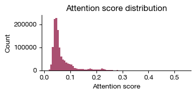
[i] attention-score distribution skewness = 3.4972.
[i] results stored under adata.uns["cellnest"].
[51]:
fig = expm.spatial_bin.plot_attention_distribution_cellnest(
    run_on_samples = [sample],
    key_added = 'cellnest',
    bins = 80,
    figsize = (4, 2)
)
[50]:
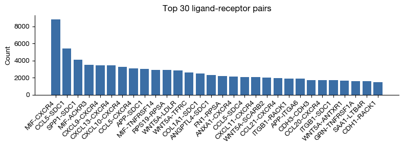
fig = expm.spatial_bin.plot_lr_frequency_cellnest(
    run_on_samples = [sample],
    key_added = 'cellnest',
    top_n = 30,
    figsize = (8, 3)
)
[49]:
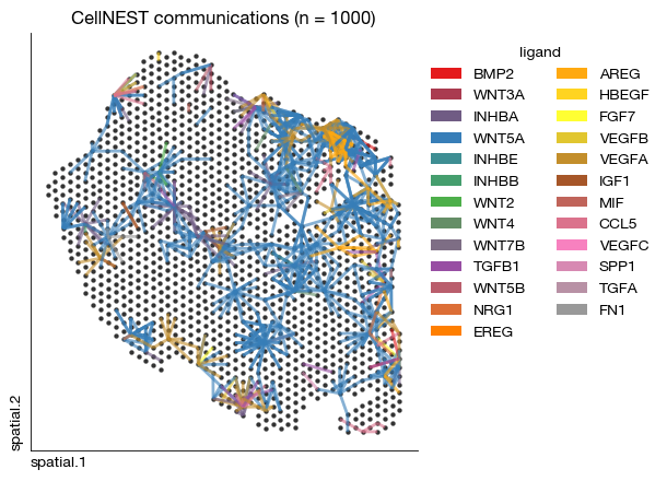
fig = expm.spatial_bin.plot_communications_cellnest(
    run_on_samples = [sample],
    key_added = 'cellnest',
    min_attention_score = 0.06,
    basis = 'spatial',
    point_color = None,
    linkage_color = 'ligand',
    linkage_cmap = 'set1',
    edge_alpha = 0.6,
    edge_width = 2,
    max_edges = 1000,
    figsize = (5.5, 4.5),
    legend_col = 2
)
[34]:
expm.spatial_bin[sample].uns['cellnest']['communications']
[34]:
| from_cell | to_cell | ligand | receptor | edge_rank | component | from_id | to_id | attention_score | |
|---|---|---|---|---|---|---|---|---|---|
| 0 | p2-t5:305 | p2-t5:317 | BMP2 | FGFR2 | 1 | -1 | 304 | 316 | 0.426324 |
| 1 | p2-t5:998 | p2-t5:635 | WNT3A | FZD2 | 2 | -1 | 997 | 634 | 0.345302 |
| 2 | p2-t5:527 | p2-t5:102 | INHBA | ACVR1B | 3 | -1 | 526 | 101 | 0.365205 |
| 3 | p2-t5:812 | p2-t5:102 | INHBA | ACVR1B | 4 | -1 | 811 | 101 | 0.367952 |
| 4 | p2-t5:1219 | p2-t5:1414 | WNT5A | TFRC | 5 | -1 | 1218 | 1413 | 0.333475 |
| ... | ... | ... | ... | ... | ... | ... | ... | ... | ... |
| 251921 | p2-t5:487 | p2-t5:559 | CCL5 | C3AR1 | 251922 | -1 | 486 | 558 | 0.162639 |
| 251922 | p2-t5:496 | p2-t5:524 | MDK | NCL | 251923 | -1 | 495 | 523 | 0.079774 |
| 251923 | p2-t5:1200 | p2-t5:1281 | JAG2 | SEC63 | 251924 | -1 | 1199 | 1280 | 0.052665 |
| 251924 | p2-t5:259 | p2-t5:48 | PIK3CB | CD247 | 251925 | -1 | 258 | 47 | 0.042083 |
| 251925 | p2-t5:306 | p2-t5:1144 | CXCL2 | C5AR1 | 251926 | -1 | 305 | 1143 | 0.127665 |
251926 rows × 9 columns
[35]:
expm.spatial_bin.cellnest_extract_relay(
    run_on_samples = [sample],
    key_added = 'cellnest',
    max_top = 200,
    score_confidence = True,
    identity = 'spagcn.refined', # cell type label
    taxa = 'hsa',
    activation_only = True
)
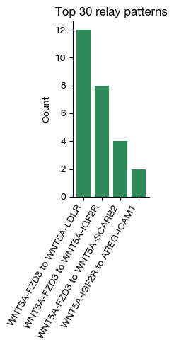
[i] extracted 4 unique 2-hop relay patterns.
[i] loading signaling and gene-regulatory networks ...
[i] pathway graph: 24754 sources, 8419668 edges, 5206 tf genes.
[i] scored 4 / 4 relays with valid paths.
[48]:
fig = expm.spatial_bin.plot_relays_cellnest(
    run_on_samples = [sample],
    key_added = 'cellnest',
    top_n = 30,
    figsize = (2.3, 5)
)
[42]:
expm.spatial_bin.view(sample)
annotated data of size 1470 × 35554
    obs : sample <cat> <c/sample> batch <cat> <c/batch> group <cat> <c> modality <cat> <c/modality>
          taxa <cat> <c/taxa> barcode <o> <o> ubc <o> <o> in.tissue <i64> <bool/intissue>
          row <i64> <f/coordinate/row> col <i64> <f/coordinate/col> y <i64> <f/coordinate/y>
          x <i64> <f/coordinate/x> leiden <cat> <c> spagcn.domain <cat> <c/domain>
          spagcn.refined <cat> <c/domain> imagerow <f64> imagecol <f64>
          deepst.domain <cat> <c/domain> deepst.refined <cat> <c/domain> integrated <cat>
          metagene.17 <f64> <f> ep1 <f32> ep2 <f32>
    var : chr <cat> <c/chromosome> start <i64> <i> end <i64> <i> strand <cat> <c/strand> id <o> <o>
          subtype <cat> <c/gsubtype> gene <cat> <o/gene> tlen <f64> <i/tlen> cdslen <i64> <i/cdslen>
          assembly <cat> <c> uid <o> <o/ugene> vst.means <f64> <f> vst.vars <f64> <f>
          vst.vars.norm <f64> <f> vst.hvg.rank <f32> <i/rank> vst.hvg <bool> <bool/hvg>
          spatialde.padj <f64> <f> spatialde.svg <bool> <bool/hvg/svg> spatialde.rank <f64> <i/rank>
 layers : counts <f32> <i/counts> imputed <f32> <f/normal> lognorm <f32> <f/normal>
          norm <f32> <f/linear>
   obsm : adjacent <arr:f64(35554)> augmented.genes <arr:f64(35554)>
          deepst.embedding <arr:f32(28)> <f/embedding> knn <arr:i32(30)> knn.d <arr:f64(30)>
          pca <arr:f64(35)> <f/embedding/pca> spatial <arr:i64(2)> <f/coordinate:2d/embedding>
          spatial.array <arr:i64(2)> tangram <df> <weights> umap <arr:f32(2)> <f/embedding>
          weights <arr:f64> cellnest.embedding <arr:f64(512)> <f/embedding>
   varm : pca <arr:f64(35)> <f/weights>
   obsp : connectivities <csr:f32> distances <csr:f64>
    uns : commands <system> deepst.domain leiden neighbors <knn> pca <dict> slots <system>
          spagcn.markers <markers> spatial <spatial> tangram <tangram> umap cellnest <cellnest>
          cellnest.relays
[47]:
expm.save()
[i] main dataset write to expm/visium/integrated.h5mu
[i] saving individual samples. (pass `save_samples = False` to skip)
━━━━━━━━━━━━━━━━━━━━━━━━ modality [spatial-bin] 8 / 8 (00:10 < 00:00)