Spot-based Spatial Profiling (ISS, ISH)#
This notebook demonstrates the analysis of spot-based spatial transcriptomics data using the exprmat package, with a focus on Xenium in-situ sequencing (ISS) and in-situ hybridization (ISH) platforms. These technologies capture gene expression at single-cell resolution directly within intact tissue sections, preserving spatial context. We work through the complete workflow from reading segmented Xenium outputs, managing large slide images through downscaling, attaching segmentation mask geometries, defining regions of interest for focused analysis, to performing clustering and annotation of cells within the tissue microenvironment.
[1]:
%load_ext autoreload
%autoreload 2
[2]:
import exprmat as em
em.setwd('../../../data')
ver = em.version()
[i] exprmat 0.2.66 / exprmat-db 0.2.66
[i] os: posix (linux)  platform version: 6.8.0-90-generic
[i] loaded configuration from /home/data/yangz/.exprmatrc
[i] current working directory: /home/data/yangz/packages/exprmat/data
[i] current database directory: /home/data/yangz/packages/database (0.2.66)
[i] resident memory: 777.75 MiB
[i] virtual memory: 5.95 GiB
Reading from segmented Xenium outputs#
Cell segmented Xenium output can be directly read to obtain the mask. For better feature support, we request the Xenium onboard analyser output cells.zarr.zip and cell_feature_matrix.zarr.zip, and recommends the morphology_focus folder be available under the repository.
If loading from transcript spots, the transcripts.parquet (or Zarr), and the morphology_focus are required since segmentation should begin with raw images.
[ ]:
meta = em.metadata(
    locations = ['./xenium'],
    modality = ['xenium/c'],
    default_taxa = ['mmu'],
    names = ['uninfected'],
    batches = ['b1'],
    groups = ['nc']
)
[4]:
expm = em.experiment(meta, dump = 'expm/xenium')
Xenium segmentation performance is commonly well. The segmentation result has been loaded into the observation matrix. However, polygonal mask need to be retrieved later using the loaded segmentation mask information.
[6]:
expm.spatial_cell['uninfected'].obs[['barcode', 'ubc', 'x', 'y', 'cid']]
[6]:
| barcode | ubc | x | y | cid | |
|---|---|---|---|---|---|
| uninfected:1 | uninfected:aaaagnff-1 | uninfected:1 | 709.756958 | 1617.774292 | 27989 |
| uninfected:2 | uninfected:aaaahafa-1 | uninfected:2 | 673.264099 | 1846.041748 | 28752 |
| uninfected:3 | uninfected:aaabgjmo-1 | uninfected:3 | 645.391602 | 1764.135620 | 92622 |
| uninfected:4 | uninfected:aaabgkok-1 | uninfected:4 | 801.664490 | 1684.112061 | 92906 |
| uninfected:5 | uninfected:aaablemm-1 | uninfected:5 | 821.919067 | 2029.243042 | 111820 |
| ... | ... | ... | ... | ... | ... |
| uninfected:219069 | uninfected:oiiklekf-1 | uninfected:219069 | 5524.763184 | 3660.229492 | 3901404325 |
| uninfected:219070 | uninfected:oiikmapd-1 | uninfected:219070 | 5502.750977 | 3662.612793 | 3901407475 |
| uninfected:219071 | uninfected:oiiknmmm-1 | uninfected:219071 | 5503.088379 | 3651.255127 | 3901414604 |
| uninfected:219072 | uninfected:oiikphad-1 | uninfected:219072 | 5513.437012 | 3658.035645 | 3901421315 |
| uninfected:219073 | uninfected:oiildplo-1 | uninfected:219073 | 5545.117676 | 3660.333008 | 3901439934 |
219073 rows × 5 columns
Rename the channel names from the default annotation to concise abbreviations. Avoid using forward slashes in channel names, as they are used as path separators within the image store hierarchy.
[8]:
expm.spatial_cell['uninfected'].uns['spatial']['uninfected']['origin']['channels'] = [
    # note that we had better change channel names to those not containing '/' char.
    'nucleus', 'membrane', '18s', 'asma-vim'
]
[9]:
expm.spatial_cell.summary(
    run_on_samples = ['uninfected']
)
uninfected
├── mask-nucleus  of shape 40865 ✗ 34148
├── mask  of shape 40865 ✗ 34148
└── origin  of shape 34148 ✗ 40865 ✗ 4
        [0] nucleus   [1] membrane  [2] 18s       [3] asma-vim
[29]:
s = 'uninfected'
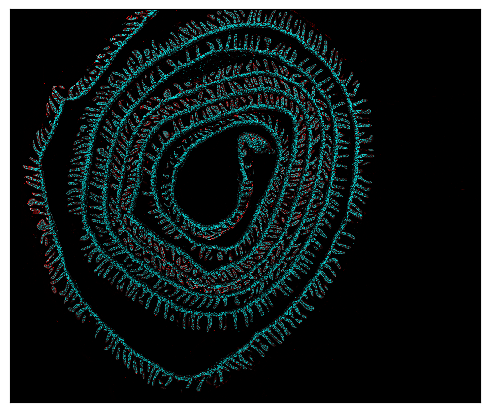
The slide image is extremely large. OpenCV did not allow loading the full size image in original resolution (image size exceeds maximum support.) It is also not a good idea to draw such large image in memory. For large-scale visualization, users should first generate a downsample of it.
Although the original OME Tiff file is pyramidal, exprmat did not load the other dimensions except the original one. For scaling to a custom downsample ratio is easy for user to carry out themselves, and program do not presumes this.
In most places of the package, channels can be specified cross-image. However, scale function is an exception, where the channels should be plain channel names inside the source image.
[15]:
expm.spatial_cell.scale(
    run_on_samples = [s],
    source = 'origin',
    destination = 'lores',
    channels = ['nucleus', 'membrane', '18s', 'asma-vim'],
    scale = 1 / 8,  # downscale 8 times
    interpolation = 2,
    xrange = None,
    yrange = None,
)
[16]:
expm.spatial_cell.summary(
    run_on_samples = [s]
)
uninfected
├── mask-nucleus  of shape 40865 ✗ 34148
├── mask  of shape 40865 ✗ 34148
├── origin  of shape 34148 ✗ 40865 ✗ 4
│       [0] nucleus   [1] membrane  [2] 18s       [3] asma-vim
└── lores  of shape 4268 ✗ 5108 ✗ 4
        [0] nucleus   [1] membrane  [2] 18s       [3] asma-vim
This plots the whole slide with low-resolution image.
[17]:
fig = expm.spatial_cell.plot_spatial(
    run_on_samples = [s],
    channels = ['lores/nucleus', 'lores/membrane'],
    channel_colors = ['cyan', 'red'],
    plot_embeddings = {
        'visible': False,
        'basis': 'spatial',
        'color': 'Foxp3'
    },
    xrange = None, yrange = None,
    figsize = (5, 5)
)
Attach segmentation mask geometries#
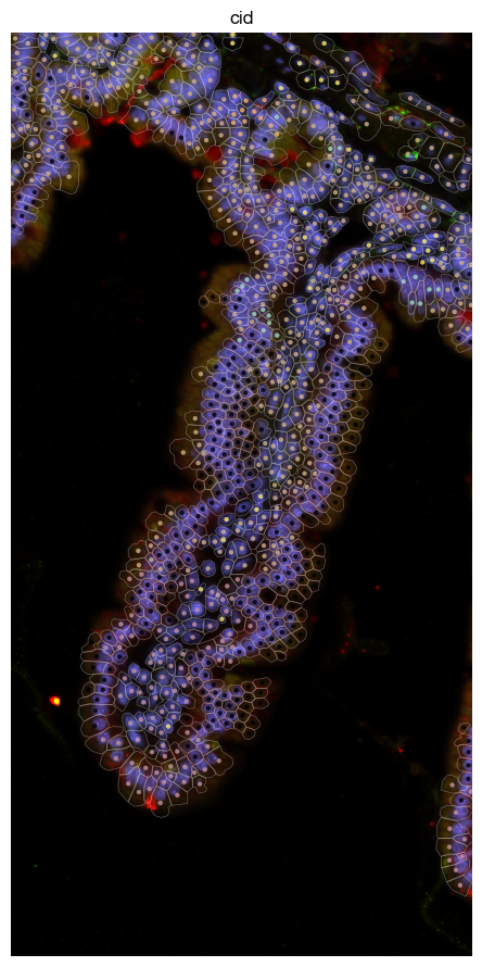
Extract polygonal cell boundaries and geometric features (area, circularity) from the segmentation mask. These geometries enable high-quality spatial visualizations where cells are displayed as polygons rather than points, and provide morphological measurements for quality control.
[24]:
expm.spatial_cell[s].obs[['x', 'y', 'area', 'cid', 'segment']]
[24]:
| x | y | area | cid | segment | |
|---|---|---|---|---|---|
| uninfected:1 | 709.756958 | 1617.774292 | 64.076721 | 27989 | 1 |
| uninfected:2 | 673.264099 | 1846.041748 | 32.060939 | 28752 | 2 |
| uninfected:3 | 645.391602 | 1764.135620 | 34.454220 | 92622 | 3 |
| uninfected:4 | 801.664490 | 1684.112061 | 38.744064 | 92906 | 4 |
| uninfected:5 | 821.919067 | 2029.243042 | 46.781877 | 111820 | 5 |
| ... | ... | ... | ... | ... | ... |
| uninfected:219069 | 5524.763184 | 3660.229492 | 32.422189 | 3901404325 | 219069 |
| uninfected:219070 | 5502.750977 | 3662.612793 | 42.582345 | 3901407475 | 219070 |
| uninfected:219071 | 5503.088379 | 3651.255127 | 109.232973 | 3901414604 | 219071 |
| uninfected:219072 | 5513.437012 | 3658.035645 | 48.859064 | 3901421315 | 219072 |
| uninfected:219073 | 5545.117676 | 3660.333008 | 26.913126 | 3901439934 | 219073 |
219073 rows × 5 columns
[30]:
fig = expm.spatial_cell.segment_features(
    run_on_samples = [s],
    mask = 'mask', correspondence = 'segment',
    key_added = 'segment'
)
━━━━━━━━━━━━━━━━━━━━━━━ extracting boundaries 219073 / 219073 (01:49 < 00:00)
[i] .obs[x] already exists, not overwriting
[i] .obs[y] already exists, not overwriting
[i] .obs[area] already exists, not overwriting
The contour geometries are now stored in obsm['segment'], providing smoothed and pixellated boundary polygons in WKT text format along with area and circularity measurements for each cell.
[31]:
expm.spatial_cell[s].obsm['segment'][['x', 'y', 'smoothened', 'area', 'circularity']]
[31]:
| x | y | smoothened | area | circularity | |
|---|---|---|---|---|---|
| uninfected:1 | 709.650756 | 1617.668102 | POLYGON ((705.713192136363 1615.8503837393368,... | 64.076726 | 0.776502 |
| uninfected:2 | 673.157839 | 1845.935533 | POLYGON ((669.1634172631815 1847.8998013044245... | 32.060941 | 0.763162 |
| uninfected:3 | 645.285392 | 1764.029447 | POLYGON ((641.1133245675701 1763.9629098112594... | 34.454223 | 0.777441 |
| uninfected:4 | 801.558221 | 1684.005884 | POLYGON ((797.9381864241273 1681.5127657720818... | 38.744067 | 0.751477 |
| uninfected:5 | 821.812826 | 2029.136981 | POLYGON ((816.4256953593247 2030.6499904416107... | 46.781881 | 0.713766 |
| ... | ... | ... | ... | ... | ... |
| uninfected:219069 | 5524.667373 | 3660.123599 | POLYGON ((5521.601009752113 3659.462960789782,... | 32.422191 | 0.937874 |
| uninfected:219070 | 5502.674307 | 3662.506674 | POLYGON ((5499.288392528724 3660.9504645551947... | 42.582349 | 0.929488 |
| uninfected:219071 | 5503.058012 | 3651.142187 | POLYGON ((5497.163493014302 3652.4500410076103... | 109.232982 | 0.851031 |
| uninfected:219072 | 5513.371747 | 3657.932404 | POLYGON ((5509.488503573921 3655.4254599734063... | 48.859068 | 0.877650 |
| uninfected:219073 | 5545.011341 | 3660.226791 | POLYGON ((5542.638415334609 3658.6129427722244... | 26.913128 | 0.861219 |
219073 rows × 5 columns
Region of interest#
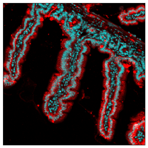
Creating regions of interest focuses on a small subset of the data
[32]:
fig = expm.spatial_cell.plot_spatial(
    run_on_samples = [s],
    channels = ['origin/nucleus', 'origin/membrane'],
    channel_colors = ['cyan', 'red'],
    channel_intensities = [1, 5],
    plot_embeddings = {
        'visible': False,
        'basis': 'spatial',
        'color': 'Foxp3'
    },
    xrange = (2500, 3000),
    yrange = (1500, 2000),
    figsize = (5, 5)
)
[33]:
expm.spatial_cell.roi(
    run_on_samples = [s],
    destination = 'roi-villi',
    scale = 1,
    xrange = (2500, 3000),
    yrange = (1500, 2000),
)
[i] created subset [roi-villi] from sample [uninfected]
[34]:
s = 'roi-villi'
[35]:
expm.spatial_cell.view(s)
annotated data of size 1759 × 451
    obs : sample <o> <c/sample> batch <o> <c/batch> group <o> <c> modality <o> <c/modality>
          taxa <o> <c/taxa> barcode <o> <o> ubc <o> <o> x <f64> <f/coordinate/x>
          y <f64> <f/coordinate/y> area <f64> <f> x.nucleus <f64> <f> y.nucleus <f64> <f>
          area.nucleus <f64> <f> z <f64> <f> n.nucleus <f64> <f> cid <ui32> <i> cid.tag <ui32> <i>
          segment <i64> <i> pixellated <o> <o/boundary> smoothened <o> <o/boundary>
          circularity <f64> <f>
    var : chr <o> <c/chromosome> start <i64> <i> end <i64> <i> strand <o> <c/strand> id <o> <o>
          subtype <o> <c/gsubtype> gene <o> <o/gene> tlen <f64> <i/tlen> cdslen <i64> <i/cdslen>
          assembly <o> <c> uid <o> <o/ugene>
   obsm : spatial <arr:f64(2)> <f/coordinate:2d/embedding> segment <df> <f>
    uns : spatial <spatial>
[36]:
expm.spatial_cell[s].obs[['x', 'y', 'area', 'cid', 'segment']]
[36]:
| x | y | area | cid | segment | |
|---|---|---|---|---|---|
| uninfected:881 | 2646.919922 | 1639.002686 | 101.150004 | 15688195 | 881 |
| uninfected:882 | 2645.441406 | 1624.791382 | 133.481880 | 15689492 | 882 |
| uninfected:883 | 2646.001709 | 1633.072510 | 122.825004 | 15700555 | 883 |
| uninfected:884 | 2641.999756 | 1644.344604 | 42.762970 | 15707889 | 884 |
| uninfected:885 | 2650.737305 | 1649.690552 | 89.635160 | 15725245 | 885 |
| ... | ... | ... | ... | ... | ... |
| uninfected:205042 | 2534.047607 | 1797.848389 | 48.046252 | 3655955456 | 205042 |
| uninfected:205043 | 2541.711426 | 1793.143555 | 14.450001 | 3655969666 | 205043 |
| uninfected:205044 | 2534.185303 | 1790.220459 | 64.663752 | 3655989773 | 205044 |
| uninfected:205142 | 2720.277100 | 1994.548340 | 67.644065 | 3657693161 | 205142 |
| uninfected:205143 | 2720.382568 | 1999.192993 | 10.250469 | 3657720339 | 205143 |
1759 rows × 5 columns
[37]:
fig = expm.spatial_cell.plot_spatial(
    run_on_samples = [s],
    channels = [
        'origin/nucleus',
        'origin/membrane',
        'origin/18s',
        'origin/asma-vim'
    ],
    channel_colors = [
        "#6b6bff",
        '#ff0000',
        '#ffff00',
        '#00ff00'
    ],
    plot_embeddings = {
        'visible': True,
        'basis': 'spatial',
        'color': 'cid',
        'ticks': True,
        'cmap': 'set3'
    },
    plot_cells = {
        'visible': True,
        # plot cell boundary
        'key_boundary': 'smoothened',
        'color': 'cid',
        'subset': None,
        'alpha': 0.3,
        'filled': False,
        'palette': 'turbo',
        'legend': False,
    },
    xrange = (2600, 2850),
    yrange = (1500, 2000),
    ticks = True,
    figsize = (6, 9), dpi = 100,
)
Clustering and annotation#
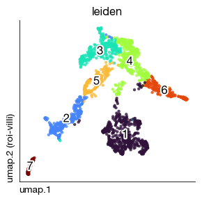
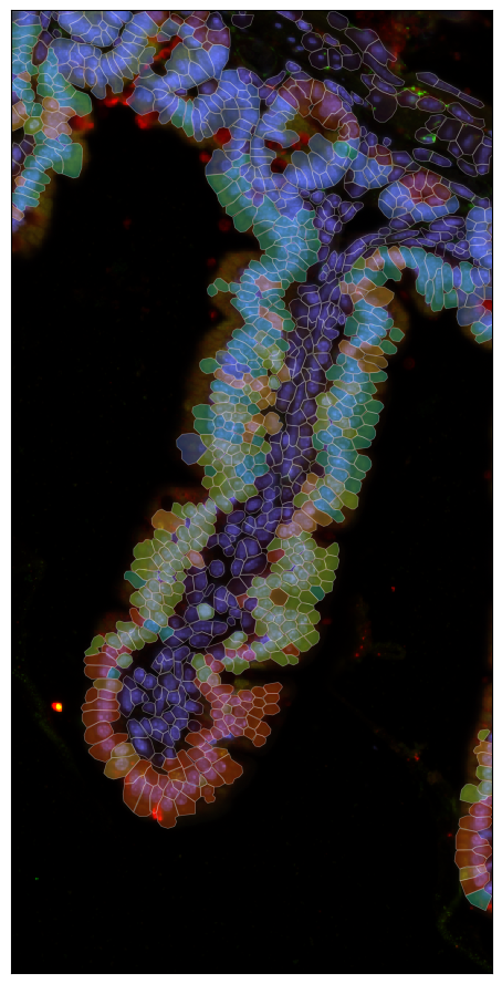
After preparing the ROI with segmentation geometries and a downscaled image, we perform standard single-cell-style analysis on the Xenium cells: log-normalization, HVG selection, PCA, KNN graph construction, Leiden clustering, and UMAP embedding. The resulting clusters are visualized both in UMAP space and overlaid on the tissue image to reveal the spatial organization of transcriptional populations.
[ ]:
expm.spatial_cell.log_normalize(
    run_on_samples = [s],
    key_norm = 'norm',
    key_lognorm = 'lognorm'
)
[39]:
expm.spatial_cell.select_hvg(
    run_on_samples = [s],
    key_lognorm = 'lognorm',
    method = 'vst',
    dest = 'vst',
    n_top_genes = 200
)
[40]:
expm.spatial_cell.scale_pca(
    run_on_samples = [s],
    hvg = 'vst.hvg',
    key_lognorm = 'lognorm',
    key_scaled = 'scaled',
    key_added = 'pca', n_comps = 35,
    keep_sparse = True,
    random_state = 42,
    svd_solver = 'arpack'
)
[41]:
expm.spatial_cell.knn(
    run_on_samples = [s],
    use_rep = 'pca',
    n_comps = None,
    n_neighbors = 30,
    knn = True,
    method = "umap",
    transformer = None,
    metric = "euclidean",
    metric_kwds = {},
    random_state = 42,
    key_added = 'neighbors',
    use_gpu = True
)
[42]:
expm.spatial_cell.leiden(
    run_on_samples = [s],
    resolution = 0.5,
    restrict_to = None,
    random_state = 42,
    key_added = 'leiden',
    adjacency = None,
    directed = None,
    use_weights = True,
    n_iterations = 2,
    partition_type = None,
    neighbors_key = None,
    obsp = None,
    flavor = 'igraph',
    use_gpu = True
)
[43]:
expm.spatial_cell.umap(
    run_on_samples = [s],
    min_dist = 0.3,
    spread = 3,
    n_components = 2,
    maxiter = 2000,
    alpha = 1,
    gamma = 1,
    negative_sample_rate = 5,
    init_pos = "random",
    random_state = 42,
    a = None, b = None,
    key_added = 'umap',
    neighbors_key = "neighbors",
    use_gpu = True
)
[44]:
fig = expm.spatial_cell.plot_embedding(
    run_on_samples = ['roi-villi'],
    basis = 'umap', color = 'leiden',
    sort = True, figsize = (3, 3), dpi = 100, legend = False
)
[47]:
fig = expm.spatial_cell.plot_spatial(
    run_on_samples = ['roi-villi'],
    channels = [
        'origin/nucleus',
        'origin/membrane',
        'origin/18s',
        'origin/asma-vim'
    ],
    channel_colors = [
        "#6b6bff",
        '#ff0000',
        '#ffff00',
        '#00ff00'
    ],
    plot_embeddings = {
        'visible': False,
        'basis': 'spatial',
        'color': 'leiden',
        'ticks': True,
        'cmap': 'turbo',
        'legend': False,
        'annotate': False,
    },
    plot_cells = {
        'visible': True,
        # plot cell boundary
        'key_boundary': 'smoothened',
        'color': 'leiden',
        'subset': None,
        'alpha': 0.3,
        'filled': True,
        'palette': 'turbo',
        'legend': False,
    },
    xrange = (2600, 2850),
    yrange = (1500, 2000),
    ticks = False,
    figsize = (6, 9), dpi = 100,
)
Save experiment#
[49]:
expm.save()
[i] saving individual samples. (pass `save_samples = False` to skip)
━━━━━━━━━━━━━━━━━━━━━━━ modality [spatial-cell] 2 / 2 (00:20 < 00:00)