Quantification of mIF Images#
After cell segmentation is complete, the next step in multiplex immunofluorescence analysis is to quantify marker expression within each segmented cell and perform quality control. This notebook demonstrates the quantification workflow for mIF data using the exprmat package, continuing from a segmented CODEX experiment. We cover spillover compensation to correct for spectral overlap between fluorophores, extraction of per-cell mean intensities for each marker, computation of cell geometry features, and quality control filtering to remove debris, small artifacts, and cells with failed nuclear staining. The result is a clean cell-by-marker expression matrix ready for downstream clustering and spatial analysis.
[1]:
%load_ext autoreload
%autoreload 2
[2]:
import exprmat as em
em.setwd('../../../data')
ver = em.version()
[i] exprmat 0.2.66 / exprmat-db 0.2.66
[i] os: posix (linux)  platform version: 6.8.0-90-generic
[i] loaded configuration from /home/data/yangz/.exprmatrc
[i] current working directory: /home/data/yangz/packages/exprmat/data
[i] current database directory: /home/data/yangz/packages/database (0.2.66)
[i] resident memory: 776.44 MiB
[i] virtual memory: 5.95 GiB
Let’s continue from a segmented CODEX. This notebook demonstrates the compensations, quantification and normalization of a typical mIF (or like) dataset.
[3]:
expm = em.load_experiment('expm/codex')
━━━━━━━━━━━━━━━━━━━━━━━━━━ loading samples 2 / 2 (00:00 < 00:00)
[!] integrated mudata object is not generated.
[4]:
expm.spatial_cell.summary(run_on_samples = True)
a-10
├── adjusted  of shape 3727 ✗ 3726 ✗ 6
│       [0] cd4   [1] cd8   [2] dapi  [3] cd45  [4] cd20  [5] cd31
├── flow  of shape 3727 ✗ 3726 ✗ 4
│       [0] r            [1] g            [2] b            [3] probability
├── mask  of shape 3727 ✗ 3726
├── mixed-membrane  of shape 3727 ✗ 3726 ✗ 1
│       [0] mixed
├── origin  of shape 3727 ✗ 3726 ✗ 59
│       [ 0] dapi        [ 1] cd45        [ 2] cd11c       [ 3] bcl2        [ 4] cd90
│       [ 5] foxp3       [ 6] egfr        [ 7] p16         [ 8] pd1         [ 9] cd206
│       [10] cd45ro      [11] il10        [12] cd56        [13] cd11b       [14] cd31
│       [15] cd163       [16] cd21        [17] cd8         [18] pnad        [19] cd20
│       [20] cxcr5       [21] ki67        [22] lag3        [23] cd73        [24] cd16
│       [25] asma        [26] icos        [27] cd25        [28] coliv       [29] pdgfrb
│       [30] cd4         [31] cd68        [32] cd34        [33] vimentin    [34] podoplanin
│       [35] hladr       [36] cxcl12      [37] cd3         [38] fap         [39] cd138
│       [40] tbet        [41] periostin   [42] spp1        [43] s100a8a9    [44] clec9a
│       [45] cd45ra      [46] caix        [47] gzmb        [48] bcat        [49] sox2
│       [50] pdl1        [51] mmp9        [52] tcrgd       [53] cd38        [54] cd69
│       [55] cd15        [56] ido1        [57] mct1        [58] panck
└── segmentation-rgb  of shape 3727 ✗ 3726 ✗ 3
        [0] r  [1] g  [2] b
a-11
├── adjusted  of shape 3733 ✗ 3732 ✗ 6
│       [0] cd4   [1] cd8   [2] dapi  [3] cd45  [4] cd20  [5] cd31
├── flow  of shape 3733 ✗ 3732 ✗ 4
│       [0] r            [1] g            [2] b            [3] probability
├── mask  of shape 3733 ✗ 3732
├── mixed-membrane  of shape 3733 ✗ 3732 ✗ 1
│       [0] mixed
├── origin  of shape 3733 ✗ 3732 ✗ 59
│       [ 0] dapi        [ 1] cd45        [ 2] cd11c       [ 3] bcl2        [ 4] cd90
│       [ 5] foxp3       [ 6] egfr        [ 7] p16         [ 8] pd1         [ 9] cd206
│       [10] cd45ro      [11] il10        [12] cd56        [13] cd11b       [14] cd31
│       [15] cd163       [16] cd21        [17] cd8         [18] pnad        [19] cd20
│       [20] cxcr5       [21] ki67        [22] lag3        [23] cd73        [24] cd16
│       [25] asma        [26] icos        [27] cd25        [28] coliv       [29] pdgfrb
│       [30] cd4         [31] cd68        [32] cd34        [33] vimentin    [34] podoplanin
│       [35] hladr       [36] cxcl12      [37] cd3         [38] fap         [39] cd138
│       [40] tbet        [41] periostin   [42] spp1        [43] s100a8a9    [44] clec9a
│       [45] cd45ra      [46] caix        [47] gzmb        [48] bcat        [49] sox2
│       [50] pdl1        [51] mmp9        [52] tcrgd       [53] cd38        [54] cd69
│       [55] cd15        [56] ido1        [57] mct1        [58] panck
└── segmentation-rgb  of shape 3733 ✗ 3732 ✗ 3
        [0] r  [1] g  [2] b
[7]:
expm.spatial_cell.view('a-10')
annotated data of size 41491 × 59
    obs : segment <i32>
    var : channel <o>
    uns : spatial
After a mask is generated, mIF images require spillover compensation. This compensation process at the same time outputs quantification matrix.
[8]:
expm.spatial_cell.compensate_spillover(
    run_on_samples = True,
    channels = 'channel',
    mask = 'mask',
    key_added = 'compensated',
)
[i] running spectral compensation for 59 channels on a-10
[i] running spectral compensation for 59 channels on a-11
For cell-level segmentation, it is convenient to directly attach the segmentation features e.g. central coordinates, size, boundaries, roundness and other geometric properties of a cell’s segmentation. For low-resolution bin-level data, such segmentation features needed to be aggregated, if a high-resolution image and segmentation available. Which is not true for most of the publicly deposited data
[9]:
expm.spatial_cell.segment_features(
    run_on_samples = True
)
   ━━━━━━━━━━━━━━━━━━━━━━━━━ extracting boundaries 41491 / 41491 (00:16 < 00:00)
   ━━━━━━━━━━━━━━━━━━━━━━━━━ extracting boundaries 48517 / 48517 (00:19 < 00:00)
Where pixellated and smoothened are boundaries polygon in WKT text.
[10]:
expm.spatial_cell.view('a-10')
annotated data of size 41491 × 59
    obs : segment <i32> x <f64> y <f64> pixellated <o> smoothened <o> area <f64> circularity <f64>
    var : channel <o>
 layers : compensated <f32> means <f32>
   obsm : segment <df> spatial <arr:f64(2)>
    uns : spatial
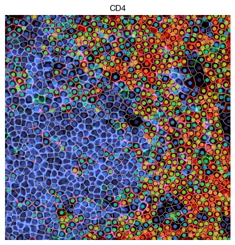
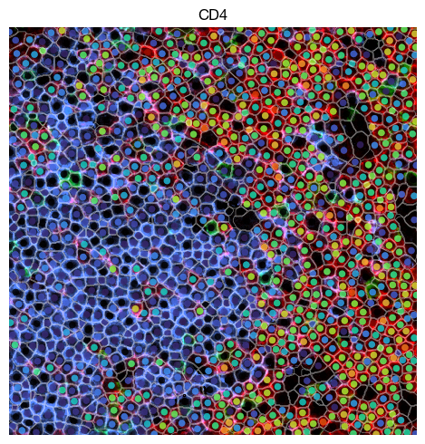
You may notice the slight but accurate differences between compensated and means
[13]:
fig = expm.spatial_cell.plot_spatial(
    run_on_samples = ['a-10'],
    channels = ['adjusted/cd4', 'adjusted/cd8', 'adjusted/cd20'],
    channel_colors = ['red', 'green', "#4c85ff"],
    plot_embeddings = {
        'visible': True,
        'color': 'CD4',
        'ptsize': 25,
        'cmap': 'turbo',
        'slot': 'means',
    },
    plot_cells = {
        'visible': True,
        # plot cell boundary
        'key_boundary': 'smoothened',
        'color': 'area',
        'subset': None,
        'alpha': 0.5,
        'filled': False,
        'palette': 'turbo',
        'legend': False,
    },
    xrange = (1500, 2000),
    yrange = (2500, 3000),
    figsize = (5, 5),
    ticks = True
)
[12]:
fig = expm.spatial_cell.plot_spatial(
    run_on_samples = ['a-10'],
    channels = ['adjusted/cd4', 'adjusted/cd8', 'adjusted/cd20'],
    channel_colors = ['red', 'green', "#4c85ff"],
    plot_embeddings = {
        'visible': True,
        'color': 'CD4',
        'ptsize': 25,
        'cmap': 'turbo',
        'slot': 'compensated',
    },
    plot_cells = {
        'visible': True,
        # plot cell boundary
        'key_boundary': 'smoothened',
        'color': 'area',
        'subset': None,
        'alpha': 0.5,
        'filled': False,
        'palette': 'turbo',
        'legend': False,
    },
    xrange = (1500, 2000),
    yrange = (2500, 3000),
    figsize = (5, 5),
    ticks = True
)
Quality control filters#
QC process filter out cells with small size, and empty nuclear signals.
[14]:
expm.spatial_cell.qc_mif(
    run_on_samples = True,
    layer = 'compensated',
    filter_max_positives = True,
    max_positive_channels_z = 3,
    filter_intensities = True,
    max_intensity_z = 3,
    filter_nuclear_staining = True,
    nuclear_staining = 'DAPI',
    min_nuclear_staining_pct = 0.01,
    filter_size = True,
    size = 'area',
    min_size_pct = 0.01,
)
[i] nuclear staining filter: 415 / 41491 cells removed (lowest 0.0100 by DAPI)
[i] size filter: 415 / 41491 cells removed (lowest 0.0100 by area)
[i] max positives filter: 0 / 41491 cells removed (n_positive z > 3)
[i] total intensity filter: 204 / 41491 cells removed (total z > 3)
[i] mif_qc: 40485 / 41491 cells passed qc
[i] nuclear staining filter: 486 / 48517 cells removed (lowest 0.0100 by DAPI)
[i] size filter: 486 / 48517 cells removed (lowest 0.0100 by area)
[i] max positives filter: 0 / 48517 cells removed (n_positive z > 3)
[i] total intensity filter: 169 / 48517 cells removed (total z > 3)
[i] mif_qc: 47396 / 48517 cells passed qc
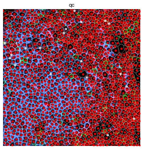
You may notice the white spots indicating artifacts that fails QC.
[15]:
fig = expm.spatial_cell.plot_spatial(
    run_on_samples = ['a-10'],
    channels = ['adjusted/cd4', 'adjusted/cd8', 'adjusted/cd20'],
    channel_colors = ['red', 'green', "#4c85ff"],
    plot_embeddings = {
        'visible': True,
        'color': 'qc',
        'ptsize': 25,
        'cmap': 'turbo',
        'slot': 'compensated',
    },
    plot_cells = {
        'visible': True,
        # plot cell boundary
        'key_boundary': 'smoothened',
        'color': 'area',
        'subset': None,
        'alpha': 0.5,
        'filled': False,
        'palette': 'turbo',
        'legend': False,
    },
    xrange = (1500, 2000),
    yrange = (2500, 3000),
    figsize = (5, 5),
    ticks = True
)
[16]:
expm.spatial_cell.filter(
    run_on_samples = True,
)
[17]:
expm.save()
[i] saving individual samples. (pass `save_samples = False` to skip)
━━━━━━━━━━━━━━━━━━━━━━━ modality [spatial-cell] 2 / 2 (00:02 < 00:00)