Profiling Clusters#
After clustering single-cell RNA-seq data into discrete populations, the next essential step is to profile each cluster by identifying its defining molecular characteristics. This notebook demonstrates how to use the exprmat package for comprehensive cluster profiling, including the identification of cluster-specific marker genes through differential expression testing, visualization of marker gene expression patterns across clusters, and functional annotation of cluster signatures. These profiling approaches facilitate biological interpretation of clustering results, enabling the assignment of cell type identities and the discovery of novel or rare subpopulations within heterogeneous tissues.
The following methods can be used to describe and characterize cluster features:
Finding marker genes, which serves as the foundation for all other methods. These are genes that are particularly highly or lowly expressed in a cluster of interest. After obtaining marker genes, you can examine them directly and look for signatures. For well-known cell type classifications, manual identification using prior knowledge is often the most convenient and quickest approach. However, prior knowledge carries the risk of error.
Gene set enrichment analysis, which uses gene sets associated with known functions to determine whether marker genes appear more or less frequently in a gene set than expected by random chance, indicating that the cluster’s characteristics are related to the functional annotation of that gene set. This provides an automated annotation method, but requires ensuring that the gene sets meet the necessary criteria. Such methods include ORA, GSEA, GSVA, and basic rank-score methods.
Homology-based annotation, if the species you are studying lacks well-annotated gene sets, or if the cell type to be identified is not well-defined, you may be able to borrow knowledge from other species. Due to the complexity of evolutionary relationships, sequence-homologous genes may no longer perform their original functions.
We will load the data directly from the integrated dataset:
[1]:
%load_ext autoreload
%autoreload 2
[2]:
import exprmat as em
# set working directory
em.setwd('../../../data')
ver = em.version()
[i] exprmat 0.2.66 / exprmat-db 0.2.66
[i] os: posix (linux)  platform version: 6.8.0-90-generic
[i] loaded configuration from /home/data/yangz/.exprmatrc
[i] current working directory: /home/data/yangz/packages/exprmat/data
[i] current database directory: /home/data/yangz/packages/database (0.2.66)
[i] resident memory: 774.93 MiB
[i] virtual memory: 5.95 GiB
[3]:
expm = em.load_experiment('expm/scrna', load_samples = False, load_subset = 'mono-neutro')
[!] samples are not dumped in the experiment directory.
[5]:
print(expm)
annotated data of size 9754 × 19651
subset mono-neutro of size 9754 × 19651
contains modalities: rna

 modality [rna]
    obs : sample <cat> <c/sample> batch <cat> <c/batch> group <cat> <c> modality <cat> <c/modality>
          taxa <cat> <c/taxa> barcode <o> <o> ubc <o> <o> n.umi <f64> <i> n.genes <i64> <i>
          n.mito <f64> <f> n.ribo <f64> <f> pct.mito <f64> <f> pct.ribo <f64> <f>
          filter <bool> <bool> score.doublet <f64> <f> score.doublet.se <f64> <f>
          is.doublet <bool> <bool> qc <bool> <bool/qc> leiden <cat> <c> sc3.5 <cat> <c>
          sc3.10 <cat> <c> sc3.20 <cat> <c> sc3.30 <cat> <c> cell.type <cat> <c>
          kde.umap <f64> <f/kde> psbulk <cat>
    var : chr <cat> <c/chromosome> start <i64> <i> end <i64> <i> strand <cat> <c/strand> id <o> <o>
          subtype <cat> <c/gsubtype> gene <cat> <o/gene> tlen <f64> <i/tlen> cdslen <i64> <i/cdslen>
          assembly <cat> <c> uid <o> <o/ugene> vst.hvg <bool> <bool/hvg> vst.all.means <f64> <f>
          vst.all.vars <f64> <f> vst.all.vars.norm <f64> <f> vst.all.hvg.rank <f32> <f>
          vst.all.hvg <bool> <bool>
 layers : counts <f32> <i/counts> norm <f32> <f>
   obsm : cnmf.10 <df> <f/embedding/usage> harmony <arr:f32(35)> <f> knn <arr:i32(100)> <i/knni>
          knn.d <arr:f32(100)> <f/knnd> pca <arr:f64(35)> <f/embedding/pca>
          umap <arr:f32(2)> <f/embedding>
   varm : cnmf.10 <arr:f64(10)> <f/weights> cnmf.coef.10 <arr:f64(10)> <f/usage-coef>
          pca <arr:f64(35)> <f/weights>
   obsp : connectivities <csr:f32> <f/connectivity> distances <csr:f32> <f/distance>
    uns : cell.type.colors cell.type_colors cnmf <cnmf> cnmf.args <o>
          cnmf.density.10 <cnmf-density> cnmf.dist.10 <f/connectivity> cnmf.stats <cnmf-stats>
          commands <system> kde.umap <kde-stats> leiden <o> leiden.colors <o> markers <markers>
          neighbors <knn> pca <dict> sc3.10.colors <o> sc3.20.colors <o> sc3.30.colors <o>
          sc3.5.colors <o> slots <system> umap <o>

[*] samples not loaded from disk.
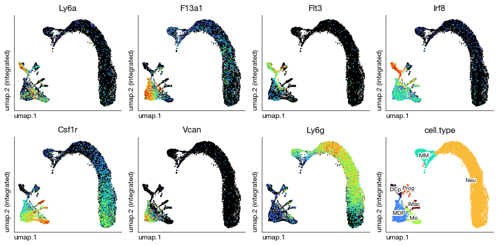
[6]:
fig = expm.rna.plot_multiple_embedding(
    basis = 'umap', features = [
        'Ly6a', 'F13a1', 'Flt3', 'Irf8',
        'Csf1r', 'Vcan', 'Ly6g', 'cell.type'
    ], ncols = 4,
    sort = True, figsize = (10, 5), dpi = 100, legend = False,
    annotate_style = 'text', annotate_fontsize = 8, ptsize = 2
)
[7]:
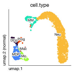
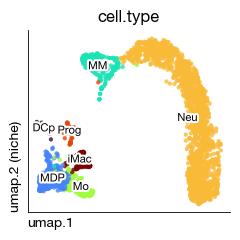
fig = expm.rna.plot_embedding(
    basis = 'umap', color = 'cell.type',
    legend = False,
    annotate = True, annotate_style = 'text', annotate_fontsize = 8,
    contour_plot = False,
    sort = True, figsize = (2.5, 2.5), dpi = 100,
    run_on_splits = True, split_key = 'sample', split_selection = ['normal', 'niche']
)
Finding marker genes#
The markers subroutine can be used to obtain differentially expressed genes of a subpopulation relative to others (or another subpopulation).
[8]:
expm.rna.markers(
    groupby = 'cell.type',
    mask_var = None,
    groups = ['Neu'],
    reference = 'rest',
    n_genes = None, rankby_abs = False, pts = True,
    key_added = 'deg.c7',
    method = 't-test',
    corr_method = 'benjamini-hochberg',
    tie_correct = False,
    gene_symbol = 'gene',
    layer = 'X'
)
[11]:
expm.rna.get_markers(
    slot = 'deg.c7',
    min_pct = 0.5,
    max_pct_reference = 0.75,
    max_q = 0.05,
    min_lfc = 1.0, max_lfc = 25,
    remove_zero_pval = False
)[['names', 'lfc', 'q', 'pct', 'pct.reference', 'log10.q', 'gene']]
[i] fetched diff `Neu` over `rest` (302 genes)
[11]:
| names | lfc | q | pct | pct.reference | log10.q | gene | |
|---|---|---|---|---|---|---|---|
| 0 | rna:mmu:g34454 | 5.000824 | 0.000000e+00 | 0.968536 | 0.358268 | 300.000000 | Mmp9 |
| 2 | rna:mmu:g1350 | 5.083699 | 0.000000e+00 | 0.917238 | 0.192585 | 300.000000 | Cxcr2 |
| 3 | rna:mmu:g48106 | 3.973207 | 0.000000e+00 | 0.974351 | 0.429462 | 300.000000 | Mxd1 |
| 4 | rna:mmu:g33362 | 4.648287 | 0.000000e+00 | 0.925291 | 0.252953 | 300.000000 | Hdc |
| 5 | rna:mmu:g31928 | 4.757430 | 0.000000e+00 | 0.780644 | 0.116142 | 300.000000 | Dhrs9 |
| ... | ... | ... | ... | ... | ... | ... | ... |
| 544 | rna:mmu:g25070 | 1.034380 | 6.239966e-111 | 0.637041 | 0.597441 | 110.204818 | Pim1 |
| 559 | rna:mmu:g1820 | 1.089561 | 1.149853e-104 | 0.634954 | 0.393701 | 103.939358 | Agap1 |
| 584 | rna:mmu:g57010 | 1.001317 | 3.344159e-99 | 0.560394 | 0.471129 | 98.475713 | Nfat5 |
| 609 | rna:mmu:g4166 | 1.012059 | 6.729340e-94 | 0.520131 | 0.377625 | 93.172028 | Hsd11b1 |
| 629 | rna:mmu:g60743 | 1.384094 | 1.305682e-89 | 0.681032 | 0.672572 | 88.884163 | Ltf |
302 rows × 7 columns
Over-representation analysis#
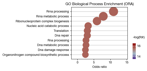
Over-representation analysis uses contingency table tests to determine whether a gene set appears more frequently in the marker gene list than expected by random chance.
[12]:
expm.rna.enrich_ora(
    taxa = 'mmu',
    de_slot = 'deg.c7', group_name = None,
    use_abs_lfc = True, min_abs_lfc = 1, max_abs_lfc = 25,
    key_added = 'ora.c7',
    gene_sets = 'bp',
    identifier = 'entrez', # the bp database contains gene names as ENTREZ
    opa_cutoff = 0.05,
)
[i] fetched diff `Neu` over `rest` (14078 genes)
[i] fetched 10675 genes differentially expressed.
[i] with a background of 18040 observed genes.
[15]:
fig = expm.rna.plot_ora_dotplot(
    slot = 'ora.c7', max_fdr = 1, max_p = 0.05,
    top_term = 10, terms = None, # draw all terms
    colour = 'fdr', cmap = 'wyj', figsize = (6, 3), cutoff = 1, ptsize = 5,

    # customizing the formatting rule of the y axis
    formatter = lambda x: x.replace('GOBP_', '').replace('_', ' ').capitalize(),
    title = 'GO Biological Process Enrichment (ORA)'
)
[i] retreived 10 terms for plotting.
Gene set enrichment analysis#
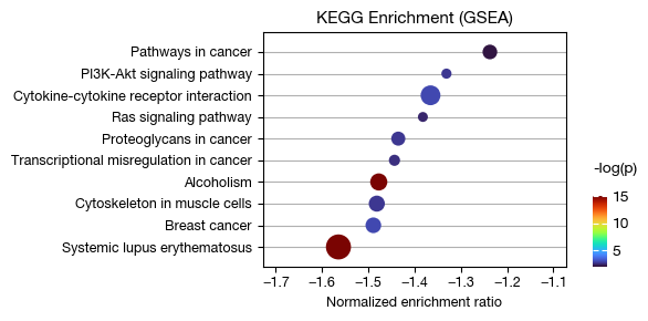
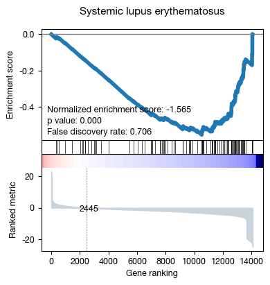
Using the log fold change of all genes between two groups, enrichment analysis can be performed via a rank-based scoring method.
[16]:
expm.rna.enrich_gsea(
    taxa = 'mmu',
    de_slot = 'deg.c7', group_name = None,
    key_added = 'gsea.c7',
    gene_sets = 'kegg',
    identifier = 'entrez'
)
[i] fetched diff `Neu` over `rest` (14078 genes)
[i] fetched 14078 preranked genes by logfc.
2026-05-11 22:17:24,363 [WARNING] Duplicated values found in preranked stats: 0.01% of genes
The order of those genes will be arbitrary, which may produce unexpected results.
[17]:
expm.rna.get_gsea(slot = 'gsea.c7')
[17]:
| name | es | nes | p | fwerp | fdr | tag | |
|---|---|---|---|---|---|---|---|
| 11 | Taurine and hypotaurine metabolism | 0.689581 | 1.708751 | 0.045714 | 0.197 | 0.111763 | 4/6 |
| 10 | Taste transduction | 0.394177 | 1.501916 | 0.040816 | 0.493 | 0.120216 | 11/29 |
| 38 | Retinol metabolism | 0.452057 | 1.502266 | 0.027778 | 0.493 | 0.180089 | 9/21 |
| 17 | Virion - Human immunodeficiency virus | -0.855095 | -1.733915 | 0.009357 | 0.153 | 0.180526 | 6/7 |
| 2 | Virion - Flavivirus and Alphavirus | -0.809305 | -1.629260 | 0.020457 | 0.545 | 0.466613 | 6/7 |
| 0 | Alcoholism | -0.511439 | -1.477416 | 0.000000 | 0.988 | 0.569829 | 51/137 |
| 40 | Basal cell carcinoma | -0.595072 | -1.505842 | 0.022175 | 0.962 | 0.601898 | 10/29 |
| 3 | Cytoskeleton in muscle cells | -0.517264 | -1.481652 | 0.002008 | 0.985 | 0.603226 | 45/129 |
| 16 | Hedgehog signaling pathway | -0.586859 | -1.517746 | 0.014644 | 0.949 | 0.613821 | 9/35 |
| 35 | Breast cancer | -0.526433 | -1.489142 | 0.001004 | 0.978 | 0.630820 | 32/94 |
| 9 | DNA replication | -0.551276 | -1.431964 | 0.044421 | 1.000 | 0.641675 | 24/34 |
| 37 | Proteoglycans in cancer | -0.498521 | -1.435232 | 0.002002 | 1.000 | 0.671578 | 45/147 |
| 6 | Transcriptional misregulation in cancer | -0.499654 | -1.443439 | 0.003000 | 0.997 | 0.672297 | 34/140 |
| 23 | Biosynthesis of unsaturated fatty acids | -0.625432 | -1.524325 | 0.021459 | 0.937 | 0.680898 | 8/21 |
| 21 | ECM-receptor interaction | -0.550174 | -1.450612 | 0.025694 | 0.995 | 0.683717 | 28/43 |
| 7 | Cytokine-cytokine receptor interaction | -0.472292 | -1.365499 | 0.001001 | 1.000 | 0.687468 | 68/158 |
| 19 | Renal cell carcinoma | -0.497755 | -1.360844 | 0.044898 | 1.000 | 0.687874 | 9/61 |
| 24 | Virion - Ebolavirus, Lyssavirus and Morbillivirus | -0.700165 | -1.541392 | 0.038976 | 0.895 | 0.699155 | 6/12 |
| 41 | Focal adhesion | -0.480401 | -1.372642 | 0.009027 | 1.000 | 0.704115 | 30/140 |
| 5 | Hippo signaling pathway | -0.488351 | -1.378083 | 0.017051 | 1.000 | 0.704133 | 20/96 |
| 25 | Systemic lupus erythematosus | -0.553177 | -1.564574 | 0.000000 | 0.820 | 0.706464 | 56/103 |
| 32 | EGFR tyrosine kinase inhibitor resistance | -0.498124 | -1.366051 | 0.032587 | 1.000 | 0.713456 | 17/69 |
| 4 | PPAR signaling pathway | -0.516196 | -1.380970 | 0.041879 | 1.000 | 0.720114 | 17/48 |
| 26 | Ras signaling pathway | -0.478279 | -1.382024 | 0.004008 | 1.000 | 0.750822 | 35/162 |
| 8 | Gastric cancer | -0.494137 | -1.387209 | 0.009082 | 1.000 | 0.755987 | 29/91 |
| 39 | PI3K-Akt signaling pathway | -0.453286 | -1.331012 | 0.002000 | 1.000 | 0.763638 | 51/231 |
| 29 | Cell adhesion molecules | -0.472574 | -1.325629 | 0.029029 | 1.000 | 0.772963 | 52/100 |
| 13 | Rap1 signaling pathway | -0.461357 | -1.334247 | 0.008000 | 1.000 | 0.798483 | 33/161 |
| 33 | Pathways in cancer | -0.416376 | -1.237094 | 0.008000 | 1.000 | 0.800584 | 123/386 |
| 12 | Calcium signaling pathway | -0.448758 | -1.291423 | 0.018018 | 1.000 | 0.807508 | 58/153 |
| 14 | Ribosome | -0.444357 | -1.259575 | 0.043043 | 1.000 | 0.836399 | 105/128 |
| 28 | MAPK signaling pathway | -0.421247 | -1.228006 | 0.027000 | 1.000 | 0.839601 | 48/224 |
[19]:
fig = expm.rna.plot_gsea_dotplot(
    slot = 'gsea.c7', max_fdr = 1, max_p = 0.05,
    top_term = 10, terms = None, # draw all terms
    colour = 'p', cmap = 'turbo', figsize = (6, 3), cutoff = 1, ptsize = 5,

    # customizing the formatting rule of the y axis
    formatter = lambda x: x,
    title = 'KEGG Enrichment (GSEA)'
)
[i] retreived 10 terms for plotting.
[22]:
fig = expm.rna.plot_gsea_leading_edge(
    slot = 'gsea.c7',
    terms = 'Systemic lupus erythematosus',
    figsize = (4, 4),
    title = None,
)
Single-cell gene set scoring#
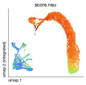
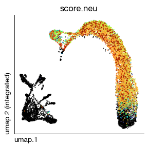
Single-cell scoring functions can be used to assess the enrichment level of specific gene sets in individual cells. score_genes is a scanpy-compatible version, while other algorithmic implementations include aucell, ulm, and gsva. These functions generate obs columns named score.{geneset}.
[27]:
expm.rna.score_genes(
    taxa = 'mmu',
    gene_sets = {
        'neu': ['S100a8', 'S100a9', 'Mpo'],
    },
    identifier = 'gene', # can be 'gene', 'uppercase', 'entrez', and 'ugene'
    lognorm = 'X',
    random_state = 42,
)
[29]:
expm['rna'].obs[['score.neu']]
[29]:
| score.neu | |
|---|---|
| distal:2 | 3.103644 |
| distal:3 | 3.853550 |
| distal:4 | 4.015083 |
| distal:8 | 3.794824 |
| distal:9 | 3.864962 |
| ... | ... |
| normal:4657 | 0.530043 |
| normal:4658 | 4.420076 |
| normal:4660 | 4.017634 |
| normal:4661 | 4.039845 |
| normal:4662 | 4.271536 |
9754 rows × 1 columns
[31]:
fig = expm.rna.plot_embedding(
    basis = 'umap', color = 'score.neu',
    sort = True, figsize = (3, 3), dpi = 100, legend = False,
    annotate_style = 'text', annotate_fontsize = 8, ptsize = 2
)
[12]:
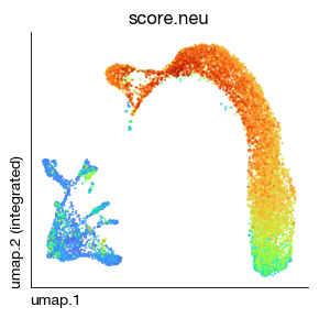
expm.rna.score_ulm(
    taxa = 'mmu',
    gene_sets = {
        'neu': ['S100a8', 'S100a9', 'Mpo'],
    },
    identifier = 'gene', # can be 'gene', 'uppercase', 'entrez', and 'ugene'
    lognorm = 'X',
    tmin = 0, # for small gene sets
)
[10]:
expm['rna'].obsm['score.ulm']
[10]:
| neu | |
|---|---|
| distal:2 | 14.599044 |
| distal:3 | 19.084107 |
| distal:4 | 21.918440 |
| distal:8 | 19.078472 |
| distal:9 | 20.233251 |
| ... | ... |
| normal:4657 | 4.259452 |
| normal:4658 | 22.427184 |
| normal:4660 | 19.939915 |
| normal:4661 | 20.791861 |
| normal:4662 | 20.143090 |
9754 rows × 1 columns
[14]:
print(expm)
annotated data of size 9754 × 19651
subset mono-neutro of size 9754 × 19651
contains modalities: rna

 modality [rna]
    obs : sample <cat> <c/sample> batch <cat> <c/batch> group <cat> <c> modality <cat> <c/modality>
          taxa <cat> <c/taxa> barcode <o> <o> ubc <o> <o> n.umi <f64> <i> n.genes <i64> <i>
          n.mito <f64> <f> n.ribo <f64> <f> pct.mito <f64> <f> pct.ribo <f64> <f>
          filter <bool> <bool> score.doublet <f64> <f> score.doublet.se <f64> <f>
          is.doublet <bool> <bool> qc <bool> <bool/qc> leiden <cat> <c> sc3.5 <cat> <c>
          sc3.10 <cat> <c> sc3.20 <cat> <c> sc3.30 <cat> <c> cell.type <cat> <c>
          kde.umap <f64> <f/kde> psbulk <cat> <o> score.neu <f64> <f/coordinate/score>
    var : chr <cat> <c/chromosome> start <i64> <i> end <i64> <i> strand <cat> <c/strand> id <o> <o>
          subtype <cat> <c/gsubtype> gene <cat> <o/gene> tlen <f64> <i/tlen> cdslen <i64> <i/cdslen>
          assembly <cat> <c> uid <o> <o/ugene> vst.hvg <bool> <bool/hvg> vst.all.means <f64> <f>
          vst.all.vars <f64> <f> vst.all.vars.norm <f64> <f> vst.all.hvg.rank <f32> <f>
          vst.all.hvg <bool> <bool>
 layers : counts <f32> <i/counts> norm <f32> <f>
   obsm : cnmf.10 <df> <f/embedding/usage> harmony <arr:f32(35)> <f> knn <arr:i32(100)> <i/knni>
          knn.d <arr:f32(100)> <f/knnd> pca <arr:f64(35)> <f/embedding/pca>
          umap <arr:f32(2)> <f/embedding> score.ulm <df> <f/score-matrix>
          padj.ulm <df> <f/score-pval>
   varm : cnmf.10 <arr:f64(10)> <f/weights> cnmf.coef.10 <arr:f64(10)> <f/usage-coef>
          pca <arr:f64(35)> <f/weights>
   obsp : connectivities <csr:f32> <f/connectivity> distances <csr:f32> <f/distance>
    uns : cell.type.colors <o> cell.type_colors <o> cnmf <cnmf> cnmf.args <o>
          cnmf.density.10 <cnmf-density> cnmf.dist.10 <f/connectivity> cnmf.stats <cnmf-stats>
          commands <system> kde.umap <kde-stats> leiden <o> leiden.colors <o> markers <markers>
          neighbors <knn> pca <dict> sc3.10.colors <o> sc3.20.colors <o> sc3.30.colors <o>
          sc3.5.colors <o> slots <system> umap <o> ulm <dict/scoring/score-ulm>

[*] samples not loaded from disk.
ULM scoring achieves well to produce scores in small gene set
[13]:
fig = expm.rna.plot_embedding(
    basis = 'umap', color = 'score.neu',
    sort = True, figsize = (3, 3), dpi = 100, legend = False,
    annotate_style = 'text', annotate_fontsize = 8, ptsize = 2
)
GSVA is less robust on such small geneset.
[15]:
expm.rna.score_gsva(
    taxa = 'mmu',
    gene_sets = {
        'neu': ['S100a8', 'S100a9', 'Mpo'],
    },
    identifier = 'gene', # can be 'gene', 'uppercase', 'entrez', and 'ugene'
    lognorm = 'X',
    tmin = 0, # for small gene sets
)
[16]:
fig = expm.rna.plot_embedding(
    basis = 'umap', color = 'score.neu',
    sort = True, figsize = (3, 3), dpi = 100, legend = False,
    annotate_style = 'text', annotate_fontsize = 8, ptsize = 2
)
[17]:
expm.rna.score_aucell(
    taxa = 'mmu',
    gene_sets = {
        'neu': ['S100a8', 'S100a9', 'Mpo'],
    },
    identifier = 'gene', # can be 'gene', 'uppercase', 'entrez', and 'ugene'
    lognorm = 'X',
    tmin = 0, # for small gene sets
)
[ ]:
fig = expm.rna.plot_embedding(
    basis = 'umap', color = 'score.neu',
    sort = True, figsize = (3, 3), dpi = 100, legend = False,
    annotate_style = 'text', annotate_fontsize = 8, ptsize = 2
)
Differential gene expression between groups#
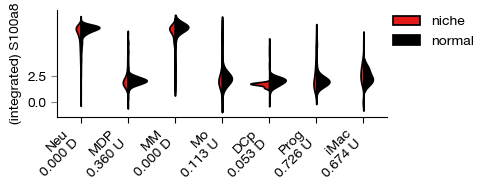
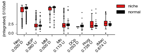
Data can be split based on two categorical variables to visualize group differences in gene expression.
[23]:
fig = expm.rna.plot_expression_bar(
    gene = 'S100a8', slot = 'X', group = 'cell.type', split = 'sample',
    selected_groups = None, selected_splits = ['niche', 'normal'], palette = ['red', 'black'],
    figsize = (5, 2), dpi = 100, style = 'violin',
    violin_kwargs = { 'split': True, 'inner': None }
)
[i] Neu, p = 0.000, D niche over normal
[i] MDP, p = 0.360, U niche over normal
[i] MM, p = 0.000, D niche over normal
[i] Mo, p = 0.113, U niche over normal
[i] DCp, p = 0.053, D niche over normal
[i] Prog, p = 0.726, U niche over normal
[i] iMac, p = 0.674, U niche over normal
[24]:
fig = expm.rna.plot_expression_bar(
    gene = 'S100a8', slot = 'X', group = 'cell.type', split = 'sample',
    selected_groups = None, selected_splits = ['niche', 'normal'], palette = ['red', 'black'],
    figsize = (5, 2), dpi = 100, style = 'box',
    violin_kwargs = { 'split': True, 'inner': None }
)
[i] Neu, p = 0.000, D niche over normal
[i] MDP, p = 0.360, U niche over normal
[i] MM, p = 0.000, D niche over normal
[i] Mo, p = 0.113, U niche over normal
[i] DCp, p = 0.053, D niche over normal
[i] Prog, p = 0.726, U niche over normal
[i] iMac, p = 0.674, U niche over normal
Saving the dataset#
Finally, save the changes we made.
[25]:
print(expm)
annotated data of size 9754 × 19651
subset mono-neutro of size 9754 × 19651
contains modalities: rna

 modality [rna]
    obs : sample <cat> <c/sample> batch <cat> <c/batch> group <cat> <c> modality <cat> <c/modality>
          taxa <cat> <c/taxa> barcode <o> <o> ubc <o> <o> n.umi <f64> <i> n.genes <i64> <i>
          n.mito <f64> <f> n.ribo <f64> <f> pct.mito <f64> <f> pct.ribo <f64> <f>
          filter <bool> <bool> score.doublet <f64> <f> score.doublet.se <f64> <f>
          is.doublet <bool> <bool> qc <bool> <bool/qc> leiden <cat> <c> sc3.5 <cat> <c>
          sc3.10 <cat> <c> sc3.20 <cat> <c> sc3.30 <cat> <c> cell.type <cat> <c>
          kde.umap <f64> <f/kde> psbulk <cat>
    var : chr <cat> <c/chromosome> start <i64> <i> end <i64> <i> strand <cat> <c/strand> id <o> <o>
          subtype <cat> <c/gsubtype> gene <cat> <o/gene> tlen <f64> <i/tlen> cdslen <i64> <i/cdslen>
          assembly <cat> <c> uid <o> <o/ugene> vst.hvg <bool> <bool/hvg> vst.all.means <f64> <f>
          vst.all.vars <f64> <f> vst.all.vars.norm <f64> <f> vst.all.hvg.rank <f32> <f>
          vst.all.hvg <bool> <bool>
 layers : counts <f32> <i/counts> norm <f32> <f>
   obsm : cnmf.10 <df> <f/embedding/usage> harmony <arr:f32(35)> <f> knn <arr:i32(100)> <i/knni>
          knn.d <arr:f32(100)> <f/knnd> pca <arr:f64(35)> <f/embedding/pca>
          umap <arr:f32(2)> <f/embedding>
   varm : cnmf.10 <arr:f64(10)> <f/weights> cnmf.coef.10 <arr:f64(10)> <f/usage-coef>
          pca <arr:f64(35)> <f/weights>
   obsp : connectivities <csr:f32> <f/connectivity> distances <csr:f32> <f/distance>
    uns : cell.type.colors cell.type_colors cnmf <cnmf> cnmf.args <o>
          cnmf.density.10 <cnmf-density> cnmf.dist.10 <f/connectivity> cnmf.stats <cnmf-stats>
          commands <system> kde.umap <kde-stats> leiden <o> leiden.colors <o> markers <markers>
          neighbors <knn> pca <dict> sc3.10.colors <o> sc3.20.colors <o> sc3.30.colors <o>
          sc3.5.colors <o> slots <system> umap <o> deg.c7 <markers> ora.c7 <ora> gsea.c7 <gsea>

[*] samples not loaded from disk.
[26]:
em.memory()
[i] resident memory: 1.94 GiB
[i] virtual memory: 18.14 GiB