Spatial Nearest Neighbor Graph#
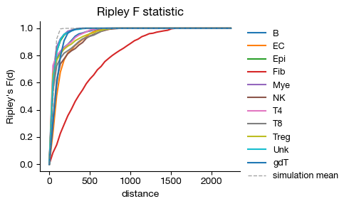
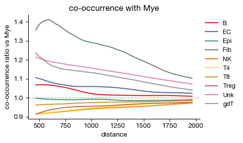
The spatial arrangement of cells within a tissue encodes critical information about tissue organization, cell-cell interactions, and the microenvironment. Spatial nearest neighbor (sNN) graphs capture these relationships by connecting each cell to its physical neighbors based on Euclidean distance in tissue coordinates. This notebook demonstrates the construction and analysis of sNN graphs for single-cell resolution spatial data using the exprmat package. We build the sNN graph, identify higher-order neighborhood structures through clustering, test for cell-type enrichment and repulsion patterns, calculate Ripley statistics for spatial point pattern analysis, and perform co-occurrence analysis to quantify how cell types are distributed relative to one another across spatial scales.
[1]:
%load_ext autoreload
%autoreload 2
[2]:
import exprmat as em
em.setwd('../../../data')
ver = em.version()
[i] exprmat 0.2.66 / exprmat-db 0.2.66
[i] os: posix (linux)  platform version: 6.8.0-90-generic
[i] loaded configuration from /home/data/yangz/.exprmatrc
[i] current working directory: /home/data/yangz/packages/exprmat/data
[i] current database directory: /home/data/yangz/packages/database (0.2.66)
[i] resident memory: 777.59 MiB
[i] virtual memory: 5.95 GiB
[3]:
expm = em.load_experiment('expm/codex')
━━━━━━━━━━━━━━━━━━━━━━━━━━ loading samples 2 / 2 (00:01 < 00:00)
[!] integrated mudata object is not generated.
[4]:
expm.spatial_cell.view('a-10')
annotated data of size 40485 × 59
    obs : segment <i32> x <f64> y <f64> pixellated <o> smoothened <o> area <f64> circularity <f64>
          qc <bool> leiden <cat> cell.type <cat>
    var : channel <o> qc <bool> vst.hvg <bool> gene <o>
 layers : compensated <f32> means <f32>
   obsm : knn <arr:i32(30)> knn.d <arr:f32(30)> pca <arr:f32(12)> segment <df> spatial <arr:f64(2)>
          umap <arr:f32(2)>
   varm : pca <arr:f64(12)>
   obsp : connectivities <csr:f32> distances <csr:f32>
    uns : leiden leiden.colors neighbors pca spatial umap
Spatial nearest neighbor graph#
[5]:
expm.spatial_cell.snn(
    run_on_samples = ['a-10'],
    key_added = 'snn',
    n_neighbors = 15,
    radius = None,
    method = 'knn',
    coord_type = 'generic'
)
[i] computing spatial neighborhood graph with knn method
[i] stored spatial neighbor graph with key_added=snn
Construct a spatial nearest neighbor (sNN) graph connecting each cell to its 15 closest neighbors based on Euclidean distance in the tissue coordinates. This graph encodes the physical tissue organization and serves as the foundation for all downstream spatial analyses.
[6]:
expm.spatial_cell.view('a-10')
annotated data of size 40485 × 59
    obs : segment <i32> x <f64> y <f64> pixellated <o> smoothened <o> area <f64> circularity <f64>
          qc <bool> leiden <cat> cell.type <cat>
    var : channel <o> qc <bool> vst.hvg <bool> gene <o>
 layers : compensated <f32> means <f32>
   obsm : knn <arr:i32(30)> knn.d <arr:f32(30)> pca <arr:f32(12)> segment <df> spatial <arr:f64(2)>
          umap <arr:f32(2)> knn.snn <arr:i64(15)> knn.d.snn <arr:f64(15)>
   varm : pca <arr:f64(12)>
   obsp : connectivities <csr:f32> distances <csr:f32> connectivities.snn <csr:f32>
          distances.snn <csr:f32>
    uns : leiden leiden.colors neighbors pca spatial umap
View the updated object to confirm that the sNN graph and connectivities have been added to the observation-level data.
[7]:
fig = expm.spatial_cell.plot_neighborhood_elbow(
    run_on_samples = ['a-10'],
    cluster_col = 'cell.type',
    connectivities_key = 'snn',
    max_neighborhoods = 30
)
[i] running elbow analysis over 1..30
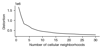
Use the elbow plot to determine the optimal number of neighborhood clusters. The plot shows how the variance explained increases with the number of neighborhoods, and the elbow point suggests a natural trade-off between resolution and interpretability.
Identifying neighborhood clusters#
[8]:
fig = expm.spatial_cell.plot_spatial(
    run_on_samples = ['a-10'],
    channels = ['adjusted/cd4', 'adjusted/cd8', 'adjusted/cd20'],
    channel_colors = ['red', 'green', "#5151ffac"],
    plot_embeddings = {
        'visible': True,
        'color': 'cell.type',
        'ptsize': 2,
        'cmap': 'turbo',
        'slot': 'compensated',
        'annotate': False,
        'legend': False
    },
    plot_cells = {
        'visible': True,
        # plot cell boundary
        'key_boundary': 'smoothened',
        'color': 'cell.type',
        'subset': None,
        'alpha': 1,
        'filled': True,
        'palette': 'turbo',
        'legend': True,
    },
    xrange = (1500, 2500),
    yrange = (2500, 3500),
    figsize = (6, 4),
    ticks = False,
    dpi = 100
)
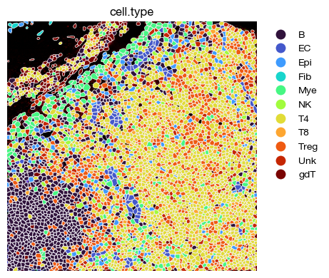
[9]:
expm.spatial_cell.neighborhood(
    run_on_samples = ['a-10'],
    cluster_col = 'cell.type',
    connectivities_key = 'snn',
    n_neighborhoods = 8,
    elbow_max = None,
    key_added = 'cneigh'
)
[i] clustering into 8 cellular neighborhoods
[10]:
fig = expm.spatial_cell.plot_spatial(
    run_on_samples = ['a-10'],
    channels = ['adjusted/cd4', 'adjusted/cd8', 'adjusted/cd20'],
    channel_colors = ['red', 'green', "#5151ffac"],
    plot_embeddings = {
        'visible': True,
        'color': 'cneigh',
        'ptsize': 2,
        'cmap': 'turbo',
        'slot': 'compensated',
        'annotate': False,
        'legend': False
    },
    plot_cells = {
        'visible': True,
        # plot cell boundary
        'key_boundary': 'smoothened',
        'color': 'cneigh',
        'subset': None,
        'alpha': 1,
        'filled': True,
        'palette': 'turbo',
        'legend': True,
    },
    xrange = (1500, 2500),
    yrange = (2500, 3500),
    figsize = (6, 4),
    ticks = False,
    dpi = 100
)
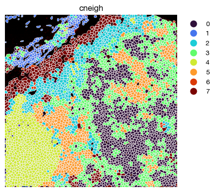
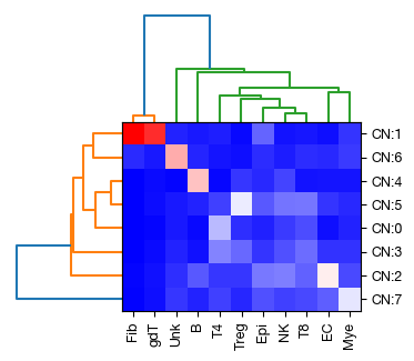
Next, we can visualize the relative composition of the neighborhoods
Visualize the composition of each neighborhood cluster as a heatmap. This reveals which cell types co-occur within the same spatial niches and defines the tissue-level organization.
[11]:
fig = expm.spatial_cell.plot_neighborhood(
    run_on_samples = ['a-10'],
    key_neighborhood = 'cneigh',
    key_cluster = 'cell.type',
    dend_x = True,
    dend_y = True,
    figsize = (3.5, 3),
    dpi = 100,
    cmap = 'bwr'
)
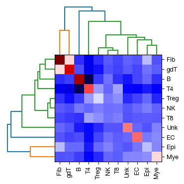
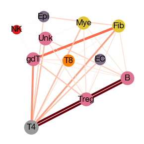
Neighborhood enrichments tests the relative normalized distance between two cell types compared to random permutation. It calculates whether cell types are closer or repelling to each other relative to random distribution.
[ ]:
expm.spatial_cell.neighborhood_enrichment(
    run_on_samples = ['a-10'],
    cluster_key = 'cell.type',
    neighbors_key = 'snn',
    n_perms = 1000,
    seed = None,
    key_added = 'nhood.enrich'
)
[i] computing observed neighbor connections
[i] computing null distribution with 1000 permutations
[i] stored nhood enrichment results in adata.uns['nhood.enrich']
[13]:
fig = expm.spatial_cell.plot_cell_type_enrichment(
    run_on_samples = ['a-10'],
    key_enrichment = 'nhood.enrich',
    key_cluster = 'cell.type',
    dend_x = True,
    dend_y = True,
    figsize = (3.5, 3.5),
    dpi = 100,
    cmap = 'seismic'
)
[14]:
fig = expm.spatial_cell.plot_cell_type_enrichment_graph(
    run_on_samples = ['a-10'],
    key_cngraph = 'nhood.enrich',
    key_cluster = 'cell.type',
    threshold = 7,
    layout = 'kk',
    node_size_factor = 40,
    edge_width_factor = 0.05,
    figsize = (3, 3),
    dpi = 100,
    cmap_node = 'set1',
    cmap_edge = 'reds/r'
)
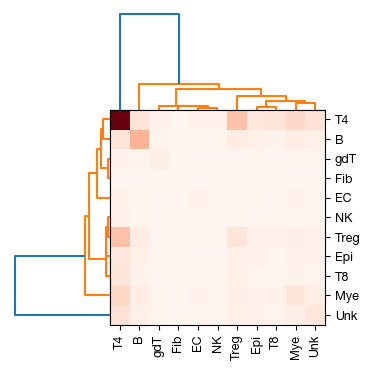
Secondary analysis to the sNN graph#
[ ]:
expm.spatial_cell.neighborhood_interaction(
    run_on_samples = ['a-10'],
    cluster_key = 'cell.type',
    neighbors_key = 'snn',
    normalized = False,
    key_added = 'interactions'
)
[i] stored interaction matrix in adata.uns['interactions']
[19]:
fig = expm.spatial_cell.plot_cell_type_interactions(
    run_on_samples = ['a-10'],
    key_interactions = 'interactions',
    key_cluster = 'cell.type',
    dend_x = True,
    dend_y = True,
    figsize = (3.5, 3.5),
    dpi = 100,
    cmap = 'reds/r'
)
[20]:
expm.spatial_cell.ripley(
    run_on_samples = ['a-10'],
    cluster_key = 'cell.type',
    mode = 'F',
    n_simulations = 100,
    n_observations = 1000,
    max_dist = None,
    n_steps = 50,
    n_neigh = 2,
    seed = 42,
    key_added = 'ripley'
)
[i] calculating ripley F statistic for 11 clusters and 100 simulations
[i] stored ripley results in adata.uns['ripley']
[21]:
fig = expm.spatial_cell.plot_ripley(
    run_on_samples = ['a-10'],
    key_added = 'ripley',
    mode = 'F',
    key_cluster = 'cell.type',
    show_sims = True,
    figsize = (5, 3),
    dpi = 100,
)
[22]:
expm.spatial_cell.cooccurence(
    run_on_samples = ['a-10'],
    cluster_key = 'cell.type',
    interval = 50,
    key_added = 'cooccur'
)
[i] computing co-occurrence probabilities for 50 intervals
[i] stored co-occurrence results in adata.uns['cooccur']
[30]:
fig = expm.spatial_cell.plot_cooccurrence(
    run_on_samples = ['a-10'],
    key_added = 'cooccur',
    key_cluster = 'cell.type',
    source_cluster = 'Mye',
    figsize = (5, 3),
    dpi = 100, cmap = 'set1',
)
[29]:
expm.save()
[i] saving individual samples. (pass `save_samples = False` to skip)
━━━━━━━━━━━━━━━━━━━━━━━ modality [spatial-cell] 2 / 2 (00:02 < 00:00)