Dataset Creation and Integration

We demonstrate how to use the exprmat package to read and integrate single-cell RNA sequencing datasets. The data loading steps for other modalities are similar, with differences only in the metadata specification. Single-cell RNA sequencing data requires at least one expression matrix; however, you can attach expression matrices for different splicing states (for RNA velocity inference) or standard 10X-format CSV files for lymphocyte receptor lineage tracing as non-independent modalities, enabling methods related to TCR/BCR clonotypes. Here we demonstrate the processing pipeline on an example dataset.

%load_ext autoreload
%autoreload 2

import exprmat as em

Importing the package

First, import the exprmat package and set the working directory to the data root.

You can use the em.version and em.cuda utility functions to check the currently installed package version. Note that the package version corresponds to the database version. The current working directory and the configured database directory will be printed. Use em.memory to check the memory usage of the current instance. em.cuda prints the list of available GPUs.

# set working directory
em.setwd('../../../data')
ver = em.version()

[i] exprmat 0.2.66 / exprmat-db 0.2.66
[i] os: posix (linux)  platform version: 6.8.0-90-generic
[i] loaded configuration from /home/data/yangz/.exprmatrc
[i] current working directory: /home/data/yangz/packages/exprmat/data
[i] current database directory: /home/data/yangz/packages/database (0.2.66)
[i] resident memory: 778.69 MiB
[i] virtual memory: 5.95 GiB

Check available GPU devices to confirm hardware acceleration is available for compute-intensive steps.

em.cuda()

[i] PyTorch version: 2.9.1+cu128
[i] GPU acceleration availability: YES
[i] CUDA version: 12.8
[i] Number of installed GPUs: 1
[i] Supporting BF16 format: YES
[i] Devices:
[i] [0] NVIDIA GeForce RTX 4090 D *
[i]     CUDA capability: (8, 9)
[i]     Installed VRAM (GiB): 47.37 GiB
[i]     Supporting TensorCore: YES
[i]     Current dedicated memory: 0.00 / 47.37 GiB (0.0%)

scRNA-seq Secondary Data with Expression Matrix Only

We create the metadata. In most cases, only secondary data are available for scRNA-seq. We consider this simplest scenario. The metadata table registers a set of 10X 3′-end single-cell RNA sequencing data from mouse bone marrow (from Cell, Volume 188, Issue 22, 6335–6354.e26). This is a labeling experiment in which whole bone marrow cells were processed without mechanical dissociation, so only hematopoietic cells are maximally retained, and no lineage-specific sorting was performed.

meta = em.metadata(
    locations    = [
        'scrna/bm-distal',
        'scrna/bm-niche',
        'scrna/bm-normal'
    ],
    modality     = ['rna', 'rna', 'rna'],
    default_taxa = ['mmu', 'mmu', 'mmu'],
    batches      = ['b1', 'b2', 'b3'],
    names        = ['distal', 'niche', 'normal'],
    groups       = ['distal', 'niche', 'normal']
)

Inspect the metadata table to verify that all sample paths, modality assignments, taxa, and batch/group labels are correctly specified before constructing the experiment object.

meta.dataframe

	location	sample	batch	group	modality	taxa
0	scrna/bm-distal	distal	b1	distal	rna	mmu
1	scrna/bm-niche	niche	b2	niche	rna	mmu
2	scrna/bm-normal	normal	b3	normal	rna	mmu

Once we confirm the metadata table has no errors, we pass it to the em.experiment constructor. The first argument is the metadata table, and the second argument tells the program the default location to save the experiment dataset.

expm = em.experiment(meta, dump = 'expm/scrna')

[i] reading sample distal [rna] ...
[i] 285 genes (out of 31053) not in the reference gene list.
[i] total 30768 genes mapped. 30748 unique genes.
[i] reading sample niche [rna] ...
[i] 285 genes (out of 31053) not in the reference gene list.
[i] total 30768 genes mapped. 30748 unique genes.
[i] reading sample normal [rna] ...
[i] 285 genes (out of 31053) not in the reference gene list.
[i] total 30768 genes mapped. 30748 unique genes.

Print the experiment summary to verify that all three samples and their RNA modality are registered correctly under the expected taxa.

print(expm)

[!] dataset not integrated.
[*] composed of samples:
  distal   rna   mmu    batch b1      of size 6654 × 30748
  niche    rna   mmu    batch b2      of size 3959 × 30748
  normal   rna   mmu    batch b3      of size 4662 × 30748

expm.rna.view('distal')

annotated data of size 6654 × 30748
    obs : sample <cat> <c/sample> batch <cat> <c/batch> group <cat> <c> modality <cat> <c/modality>
          taxa <cat> <c/taxa> barcode <o> <o> ubc <o> <o>
    var : chr <cat> <c/chromosome> start <i64> <i> end <i64> <i> strand <cat> <c/strand> id <o> <o>
          subtype <cat> <c/gsubtype> gene <cat> <o/gene> tlen <f64> <i/tlen> cdslen <i64> <i/cdslen>
          assembly <cat> <c> uid <o> <o/ugene>
    uns : commands <system> slots <system>

Quality Control

Next, we perform quality control on the data. The initial QC steps for single-cell RNA sequencing are performed independently on each sample. These include removing empty droplets, filtering cells with too few detected genes, filtering cells with a high proportion of mitochondrial transcripts, and inferring and removing doublets. Because each sample is independent, the same QC operations can be parallelized across samples using the parallel parameter for multiprocessing, which can substantially speed up processing (roughly 5-fold). However, for a small number of samples, parallelization offers little benefit, so we use synchronous execution here.

expm.rna.qc(
    run_on_samples = True,
    mt_seqid = 'chrM',
    mt_percent = 0.15,
    ribo_genes = None,
    ribo_percent = None,
    outlier_mode = 'mads',
    outlier_n = 5,
    doublet_method = 'scrublet',
    min_cells = 3,
    min_genes = 600,
    parallel = 2
)

   ━━━━━━━━━━━━━━━━━━━━━━━━━━ processing samples       3 / 3     (00:13 < 00:00)

Print the updated experiment summary to confirm that QC flags, doublet scores, and filtering annotations have been applied to each sample’s observation table.

print(expm)

[!] dataset not integrated.
[*] composed of samples:
  distal   rna   mmu    batch b1      of size 6451 × 21689
  niche    rna   mmu    batch b2      of size 3656 × 21970
  normal   rna   mmu    batch b3      of size 4537 × 21917

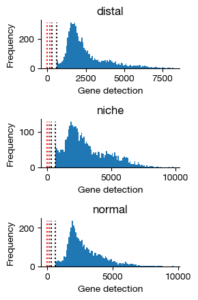
Here, we will have a glance at the distribution of detected genes per cell. Typically, this will be a zero-inflated normal distribution. The four marker lines indicates 0, 100, 300 and 600 genes of the X axis.

gene_counts = expm.rna.plot_gene_histograms(ncols = 1, figsize = (3, 4.5))

Plot multi-panel QC figures for each sample, showing total counts, number of detected genes, mitochondrial fraction, and doublet scores. These diagnostic plots guide the selection of filtering thresholds and help identify problematic samples before downstream analysis.

figs = expm.rna.plot_qc(run_on_samples = True, figsize = (10, 2.2))

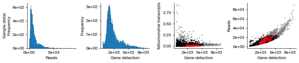
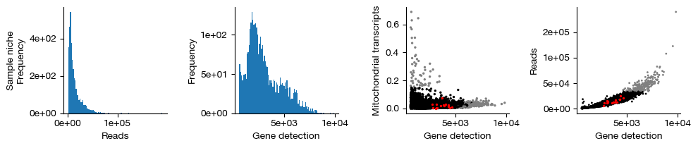
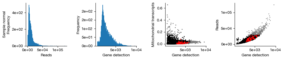
Finally, we retain only the cells that passed QC (shown in black in the figure above; red indicates inferred doublets, and gray indicates cells filtered out due to failing gene count, transcript count, or mitochondrial transcript proportion thresholds). This operation permanently removes these cells from each sample and is irreversible. We do not use .raw to preserve the unfiltered cells.

expm.save()
expm.rna.filter(run_on_samples = True)

Per-sample Data Processing

For thorough data processing, we first inspect the data quality at the individual sample level to identify and exclude outlier samples.

expm.rna.log_normalize(
    run_on_samples = True,
    key_norm = 'norm',
    key_lognorm = 'lognorm'
)

Select the top highly variable genes per sample using the variance-stabilizing transformation (VST) method. This identifies genes with the highest residual variance after accounting for the mean-variance relationship, focusing downstream analysis on the most informative features.

expm.rna.select_hvg(
    run_on_samples = True,
    key_lognorm = 'lognorm',
    method = 'vst',
    dest = 'vst',
    n_top_genes = 1500
)

Scale the log-normalized expression to unit variance (z-scoring per gene) and compute PCA on the HVG subset. The scaled data ensures that highly expressed genes do not dominate the principal components, and PCA provides a compact low-dimensional representation of the major axes of variation.

expm.rna.scale_pca(
    run_on_samples = True,
    hvg = 'vst.hvg',
    key_lognorm = 'lognorm',
    key_scaled = 'scaled',
    key_added = 'pca', n_comps = 35,
    keep_sparse = False,
    random_state = 42,
    svd_solver = 'arpack'
)

Build a k-nearest-neighbor graph on the PCA embedding using cosine distance. The KNN graph captures local cell-cell similarities and forms the basis for graph-based clustering and non-linear embedding methods.

expm.rna.knn(
    run_on_samples = True,
    use_rep = 'pca',
    n_comps = None,
    n_neighbors = 30,
    knn = True,
    method = "umap",
    transformer = None,
    metric = "cosine",
    metric_kwds = {},
    random_state = 42,
    key_added = 'neighbors',
    use_gpu = True
)

Cluster cells using the Leiden algorithm on the KNN graph. Leiden is a graph-based community detection method that iteratively optimizes modularity to find stable partitions. The resolution parameter controls the granularity of the clustering — higher values produce more clusters.

expm.rna.leiden(
    run_on_samples = True,
    resolution = 0.5,
    restrict_to = None,
    random_state = 42,
    key_added = 'leiden',
    adjacency = None,
    directed = None,
    use_weights = True,
    n_iterations = 2,
    partition_type = None,
    neighbors_key = None,
    obsp = None,
    flavor = 'igraph',
    use_gpu = True
)

Compute a 2D UMAP embedding from the KNN graph for visualization. UMAP preserves both local and global data structure, producing a layout where similar cells appear close together. The min_dist and spread parameters control the compactness of the embedding.

expm.rna.umap(
    run_on_samples = True,
    min_dist = 0.45,
    spread = 0.9,
    n_components = 2,
    maxiter = None,
    alpha = 1,
    gamma = 1,
    negative_sample_rate = 5,
    init_pos = "spectral",
    random_state = 42,
    a = None, b = None,
    key_added = 'umap',
    neighbors_key = "neighbors"
)

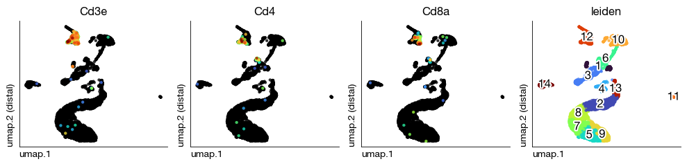
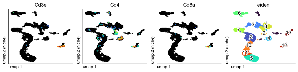
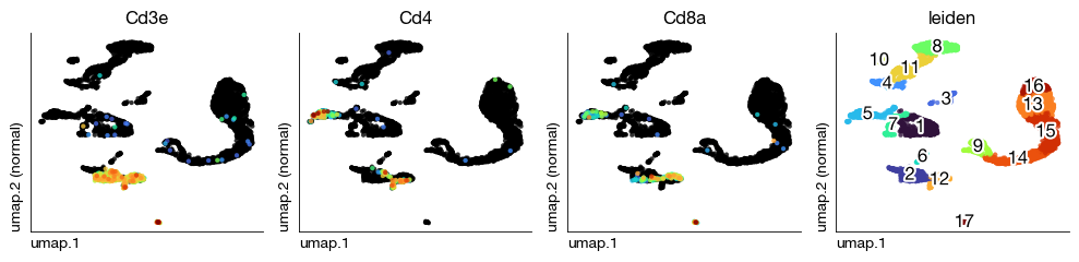
Visualize per-sample UMAPs with T cell markers and Leiden clusters to spot anomalies before integration.

figs = expm.rna.plot_multiple_embedding(
    run_on_samples = True,
    basis = 'umap', features = ['Cd3e', 'Cd4', 'Cd8a', 'leiden'], ncols = 4,
    sort = True, figsize = (10, 2.5), dpi = 100, legend = False
)

Dataset Integration

After confirming that each sample is correct and without issues, we integrate the data. This merges all samples of the same modality into a single large AnnData object. The expm.merge function performs this concatenation without altering any counts. The integrated data then requires batch correction to obtain a corrected embedding representation.

print(expm)

[!] dataset not integrated.
[*] composed of samples:
  distal   rna   mmu    batch b1      of size 5660 × 18002
  niche    rna   mmu    batch b2      of size 3297 × 18067
  normal   rna   mmu    batch b3      of size 4058 × 18377

Concatenate all per-sample AnnData objects into a single merged object using an outer join on the gene union. The variable_columns parameter preserves per-sample HVG annotations, and bool_merge_behavior='or' ensures a gene is flagged as highly variable if it was selected in any sample.

expm.merge(
    join = 'outer',
    variable_columns = ['vst.hvg'],
    bool_merge_behavior = 'or'
)

print(expm)

annotated data of size 13015 × 19651
integrated dataset of size 13015 × 19651
contains modalities: rna

 modality [rna]
    obs : sample <cat> <c/sample> batch <cat> <c/batch> group <cat> <c> modality <cat> <c/modality>
          taxa <cat> <c/taxa> barcode <o> <o> ubc <o> <o> n.umi <f64> <i> n.genes <i64> <i>
          n.mito <f64> <f> n.ribo <f64> <f> pct.mito <f64> <f> pct.ribo <f64> <f>
          filter <bool> <bool> score.doublet <f64> <f> score.doublet.se <f64> <f>
          is.doublet <bool> <bool> qc <bool> <bool/qc> leiden <cat> <c>
    var : chr <o> <c/chromosome> start <i64> <i> end <i64> <i> strand <o> <c/strand> id <o> <o>
          subtype <o> <c/gsubtype> gene <o> <o/gene> tlen <f64> <i/tlen> cdslen <i64> <i/cdslen>
          assembly <o> <c> uid <o> <o/ugene> vst.hvg <bool> <bool/hvg>
 layers : counts <f32> <i/counts>
    uns : slots <system>

[*] composed of samples:
  distal   rna   mmu    batch b1      of size 5660 × 18002
  niche    rna   mmu    batch b2      of size 3297 × 18067
  normal   rna   mmu    batch b3      of size 4058 × 18377

Re-select HVGs on the merged dataset, using batch as a covariate to find consistently variable genes.

expm.rna.select_hvg(
    key_lognorm = 'X',
    method = 'vst',
    dest = 'vst.all',
    n_top_genes = 2000,
    batch_key = 'batch',
    sort_hvg_rank_first = False,
    span = 0.3
)

Remove TCR gene segments (Trav, Trad, Traj, Trac, Trbv, Trbd, Trbj, Trbc) and ribosomal protein genes (Rpl, Rps) from the highly variable gene list. These genes tend to show high variance due to technical factors or clonal abundance rather than biologically meaningful cell-type differences, and their inclusion would distort the PCA embedding and clustering.

# exclude lateral genes from the highly variable list.
hvgs = expm.mudata['rna'].var['vst.all.hvg'].tolist()
names = expm.mudata['rna'].var['gene'].tolist()
for idx, name in enumerate(names):
    if str(name) == 'nan': continue
    if (name.startswith('Trav') or
        name.startswith('Trad') or
        name.startswith('Traj') or
        name.startswith('Trac') or
        name.startswith('Trbv') or
        name.startswith('Trbd') or
        name.startswith('Trbj') or
        name.startswith('Trbc') or
        name.startswith('Rpl') or
        name.startswith('Rps')
    ):
        hvgs[idx] = False

expm.mudata['rna'].var['vst.all.hvg'] = hvgs
expm.mudata['rna'].var['vst.all.hvg'].value_counts()

vst.all.hvg
False    17714
True      1937
Name: count, dtype: int64

Scale the expression data again and recompute PCA on the cleaned, merged HVG set. This PCA will be used as input for batch correction methods like Harmony.

expm.rna.scale_pca(
    hvg = 'vst.hvg',
    key_lognorm = 'X',
    key_scaled = 'scaled',
    key_added = 'pca', n_comps = 35,
    keep_sparse = False,
    random_state = 42,
    svd_solver = 'arpack'
)

Apply Harmony to correct batch effects in PCA space, producing a batch-corrected embedding.

expm.rna.integrate(
    method = 'harmony',
    basis = 'pca',
    dest = 'harmony'
)

2026-05-10 00:13:53,631 - harmonypy - INFO - Computing initial centroids with sklearn.KMeans...
2026-05-10 00:13:53 | [INFO] Computing initial centroids with sklearn.KMeans...
2026-05-10 00:13:53,895 - harmonypy - INFO - KMeans initialization complete.
2026-05-10 00:13:53 | [INFO] KMeans initialization complete.

Build the KNN graph on the Harmony-corrected embedding. Using Euclidean distance in the Harmony space (where batch effects have been removed) ensures that neighbors are identified based on biological similarity rather than technical origin.

expm.rna.knn(
    use_rep = 'harmony',
    n_comps = None,
    n_neighbors = 35,
    knn = True,
    method = "umap",
    transformer = None,
    metric = "euclidean",
    metric_kwds = {},
    random_state = 42,
    key_added = 'neighbors',
    use_gpu = True
)

Cluster the batch-corrected cells using Leiden on the Harmony-based KNN graph. At this resolution, the clusters should represent biologically distinct cell populations rather than batch-specific groupings.

expm.rna.leiden(
    resolution = 0.8,
    restrict_to = None,
    random_state = 42,
    key_added = 'leiden',
    adjacency = None,
    directed = None,
    use_weights = True,
    n_iterations = 2,
    partition_type = None,
    neighbors_key = None,
    obsp = None,
    flavor = 'igraph'
)

Compute the integrated UMAP embedding from the Harmony-corrected neighbor graph. This UMAP will show cells colored by biological identity rather than batch, enabling visual assessment of integration quality and the identification of shared cell types across samples.

expm.rna.umap(
    min_dist = 0.5,
    spread = 1,
    n_components = 2,
    maxiter = None,
    alpha = 1,
    gamma = 1,
    negative_sample_rate = 5,
    init_pos = "spectral",
    random_state = 0,
    a = None, b = None,
    key_added = 'umap',
    neighbors_key = "neighbors"
)

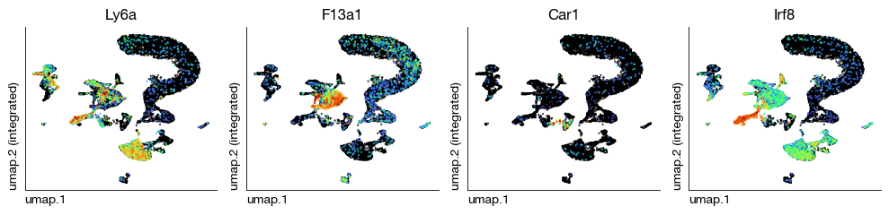
Visualize known marker genes on the integrated UMAP to verify that cell populations are correctly separated and that batch correction did not over-correct biologically meaningful variation. The expression patterns of lineage-specific markers should align with the cluster structure.

fig = expm.rna.plot_multiple_embedding(
    basis = 'umap', features = ['Ly6a', 'F13a1', 'Car1', 'Irf8'], ncols = 4,
    sort = True, figsize = (10, 2.5), dpi = 100, legend = False,
    annotate_style = 'text', annotate_fontsize = 8, ptsize = 2
)

Inspect the experiment state after Harmony integration to review the merged data dimensions and available embeddings.

print(expm)

annotated data of size 13015 × 19651
integrated dataset of size 13015 × 19651
contains modalities: rna

 modality [rna]
    obs : sample <cat> <c/sample> batch <cat> <c/batch> group <cat> <c> modality <cat> <c/modality>
          taxa <cat> <c/taxa> barcode <o> <o> ubc <o> <o> n.umi <f64> <i> n.genes <i64> <i>
          n.mito <f64> <f> n.ribo <f64> <f> pct.mito <f64> <f> pct.ribo <f64> <f>
          filter <bool> <bool> score.doublet <f64> <f> score.doublet.se <f64> <f>
          is.doublet <bool> <bool> qc <bool> <bool/qc> leiden <cat> <c>
    var : chr <o> <c/chromosome> start <i64> <i> end <i64> <i> strand <o> <c/strand> id <o> <o>
          subtype <o> <c/gsubtype> gene <o> <o/gene> tlen <f64> <i/tlen> cdslen <i64> <i/cdslen>
          assembly <o> <c> uid <o> <o/ugene> vst.hvg <bool> <bool/hvg> vst.all.means <f64>
          vst.all.vars <f64> vst.all.vars.norm <f64> vst.all.hvg.rank <f32> vst.all.hvg <bool>
 layers : counts <f32> <i/counts>
   obsm : pca <arr:f64(35)> <f/embedding/pca> harmony <arr:f32(35)> knn <arr:i32(35)>
          knn.d <arr:f32(35)> umap <arr:f32(2)> <f/embedding>
   varm : pca <arr:f64(35)> <f/weights>
   obsp : connectivities <csr:f32> distances <csr:f32>
    uns : slots <system> commands <system> pca <dict> neighbors <knn> leiden umap

[*] composed of samples:
  distal   rna   mmu    batch b1      of size 5660 × 18002
  niche    rna   mmu    batch b2      of size 3297 × 18067
  normal   rna   mmu    batch b3      of size 4058 × 18377

Dataset Integration Using scVI

When cell type distributions are highly imbalanced across samples, integration methods based on MNN or Harmony tend to artificially merge distinct cell types together, leading to uninterpretable results. The scVI method handles this better, especially when you need to integrate sequencing data generated under different sorting strategies into a relatively unbiased dataset.

Train the scVI variational inference model on the merged dataset using raw UMI counts. scVI uses a deep probabilistic framework that models count distributions with a zero-inflated negative binomial likelihood, accounting for library size differences and batch effects through latent variables. The model learns a low-dimensional latent representation that captures biological variation while removing technical artifacts. Training parameters like n_hidden, n_layers, and dropout_rate control the neural network architecture and regularization.

expm.rna.scvi(
    batch = 'batch', n_comps = 30,
    hvg = 'vst.hvg', key_counts = 'counts',
    key_added = 'scvi',

    # seeding options, if you have a semi-annotated data
    seeding = False,
    imputed_label_key = None,

    # parameters passed to scvi
    n_hidden = 128,
    n_layers = 3,
    dropout_rate = 0.1,
    dispersion = "gene",
    gene_likelihood = "zinb",
    use_observed_lib_size = True,
    latent_distribution = "normal",
    max_epochs = None,
)

Build the KNN graph on the scVI latent space. Using the full scVI embedding (all 30 dimensions) with Euclidean distance ensures that the neighbor graph reflects the denoised, batch-corrected representation learned by the deep generative model.

expm.rna.knn(
    use_rep = 'scvi',
    n_comps = None,
    n_neighbors = 50,
    knn = True,
    method = "umap",
    transformer = None,
    metric = "euclidean",
    metric_kwds = {},
    random_state = 42,
    key_added = 'nn.scvi',
    use_gpu = True
)

Compute UMAP from the scVI-based neighbor graph. Comparing this embedding to the Harmony-based UMAP helps evaluate which integration method better preserves biological structure for the specific dataset characteristics.

expm.rna.umap(
    min_dist = 0.35,
    spread = 1,
    n_components = 2,
    maxiter = None,
    alpha = 1,
    gamma = 1,
    negative_sample_rate = 5,
    init_pos = "spectral",
    random_state = 80,
    a = None, b = None,
    key_added = 'umap',
    neighbors_key = "nn.scvi"
)

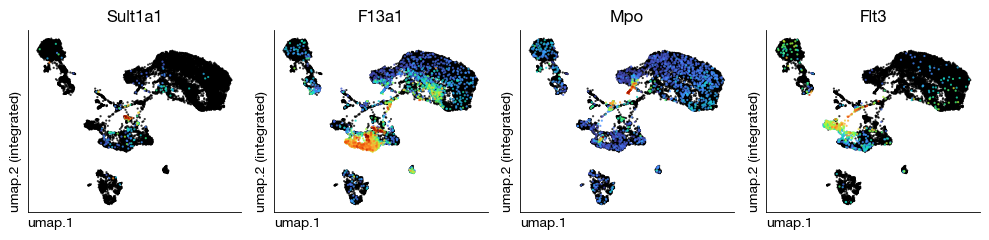
Visualize the scVI-integrated UMAP with cell-type-specific marker genes to assess whether the integration preserved known biological distinctions. Compare these expression patterns with the Harmony results to determine which method provides cleaner separation for the dataset.

fig = expm.rna.plot_multiple_embedding(
    basis = 'umap', features = ['Sult1a1', 'F13a1', 'Mpo', 'Flt3'], ncols = 4,
    sort = True, figsize = (10, 2.5), dpi = 100, legend = False,
    annotate_style = 'text', annotate_fontsize = 8, ptsize = 2
)

Print the final experiment summary after scVI integration, verifying that all embeddings, cluster assignments, and additional data slots are properly stored.

print(expm)

annotated data of size 13015 × 19651
integrated dataset of size 13015 × 19651
contains modalities: rna

 modality [rna]
    obs : sample <cat> <c/sample> batch <cat> <c/batch> group <cat> <c> modality <cat> <c/modality>
          taxa <cat> <c/taxa> barcode <o> <o> ubc <o> <o> n.umi <f64> <i> n.genes <i64> <i>
          n.mito <f64> <f> n.ribo <f64> <f> pct.mito <f64> <f> pct.ribo <f64> <f>
          filter <bool> <bool> score.doublet <f64> <f> score.doublet.se <f64> <f>
          is.doublet <bool> <bool> qc <bool> <bool/qc> leiden <cat> <c>
    var : chr <o> <c/chromosome> start <i64> <i> end <i64> <i> strand <o> <c/strand> id <o> <o>
          subtype <o> <c/gsubtype> gene <o> <o/gene> tlen <f64> <i/tlen> cdslen <i64> <i/cdslen>
          assembly <o> <c> uid <o> <o/ugene> vst.hvg <bool> <bool/hvg> vst.all.means <f64>
          vst.all.vars <f64> vst.all.vars.norm <f64> vst.all.hvg.rank <f32> vst.all.hvg <bool>
 layers : counts <f32> <i/counts>
   obsm : pca <arr:f64(35)> <f/embedding/pca> harmony <arr:f32(35)> knn <arr:i32(35)>
          knn.d <arr:f32(35)> umap <arr:f32(2)> <f/embedding>
   varm : pca <arr:f64(35)> <f/weights>
   obsp : connectivities <csr:f32> distances <csr:f32>
    uns : slots <system> commands <system> pca <dict> neighbors <knn> leiden umap

[*] composed of samples:
  distal   rna   mmu    batch b1      of size 5660 × 18002
  niche    rna   mmu    batch b2      of size 3297 × 18067
  normal   rna   mmu    batch b3      of size 4058 × 18377

Saving the Dataset

To save the dataset, if save_samples is set to False, we will not save the per-sample sub-datasets, saving only the integrated data. This can save considerable time, or is useful when you do not want new modifications to overwrite previously saved samples. However, we recommend saving at least one version of the per-sample data, as they may be useful later and can avoid repeating QC operations.

expm.save(save_samples = False)

[i] main dataset write to expm/scrna/integrated.h5mu

Report current memory usage of all loaded objects to monitor resource consumption and identify potential memory bottlenecks with large datasets.

em.memory()

[i] resident memory: 3.72 GiB
[i] virtual memory: 30.83 GiB