Genome Assembly Visualization

The exprmat package bundles reference genome assemblies for human and mouse, and provides a composable set of functions for visualizing genomic tracks. These visualization tools allow researchers to inspect genomic features such as chromosome architecture, gene annotations, read coverage, and epigenetic signals across any genomic region of interest.

Background

Genome assemblies are reference sequences that represent the complete set of chromosomes for an organism. Different assemblies exist for the same species (e.g., GRCh38 vs GRCh37 for human, GRCm39 vs GRCm38 for mouse), and they differ in contiguity, error correction, and representation of difficult genomic regions. The exprmat database ships pre-processed assembly data so that genomic coordinates can be unambiguously interpreted.

The track visualization system follows the widely-used “Genome Browser” paradigm (like UCSC Genome Browser or IGV), where multiple horizontally stacked tracks share the same genomic coordinates, enabling side-by-side comparison of different data modalities.

from exprmat.plotting.track import (
    architecture,
    genes,
    initialize_tracks,
    genome_track,
    chromosome_track,
    gene_track,
    bed_track,
    coverage_track_from_bam,
    coverage_track_from_bigwig
)

Chromosome Architecture Visualization

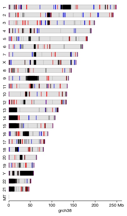
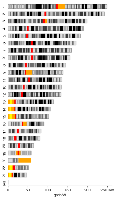
By specifying an assembly name and a coloring scheme, we can render the chromosome architecture stored in the built-in database. The cby (color by) parameter supports two options:

• assembly: Colors genomic regions according to their assembly classification. By default:

  • Fix Patches (red): Refined sequences that correct errors in the primary assembly

  • Novel Patches (blue): Alternate representations of complex loci (e.g., MHC, KIR regions)

  • Alternate Scaffolds (gray): Alternative locus representations (typically in gray)

  • Telomeres (purple): Chromosome end regions with repetitive (TTAGGG)n sequences

  • Centromeres (green): Chromosome constriction regions essential for segregation

  • Pseudoautosomal Regions (PAR) (orange): Homologous regions on sex chromosomes that recombine during male meiosis

  • Gaps (black): Unresolved stretches of unknown sequence

• cytobands: Giemsa-stained chromosome banding patterns (G-banding), a classical cytogenetic technique where:

  • Centromeres are colored red

  • Variable regions (heterochromatin) are colored orange

  • Satellite stalks (nucleolar organizer regions, NORs) are colored yellow

  • Dark G-bands represent AT-rich, gene-poor regions; light G-bands represent GC-rich, gene-dense regions

Chromosomes are arranged by size (largest first) by default. The architecture() function generates a horizontally stacked ideogram view, useful for overview figures in publications.

arch = architecture('grch38', cby = 'assembly', figsize = (4, 7))

arch = architecture('grch38', cby = 'cytobands', figsize = (4, 7))

Gene Annotation Tracks

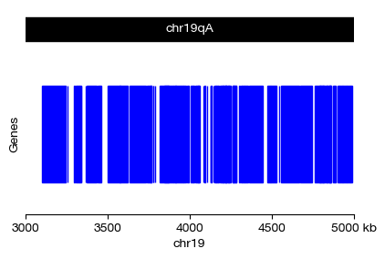
By specifying a chromosome interval (a region defined by a chromosome name, a start coordinate, and an end coordinate), we can render the annotated gene models from the reference genome. The genes() function is a convenience wrapper that automatically handles chromosome track, gene track, and coordinate axis layout.

Important rendering behavior: When more than ~20 genes are visible within the selected window, individual gene structure (exons, introns, UTRs) becomes too dense to display clearly. In such cases, the plot automatically simplifies to show only gene-level rectangles without internal exon/intron details, maintaining visual clarity at the cost of resolution.

Coordinate system: Genomic coordinates in exprmat use 0-based, half-open intervals, consistent with the BED format standard. The xfrom and xto parameters define the window [xfrom, xto).

fig = genes(
    assembly = 'grcm39',
    chr = 'chr19',
    xfrom = 3e6,
    xto = 5e6,
    figsize = (4, 2.5)
)

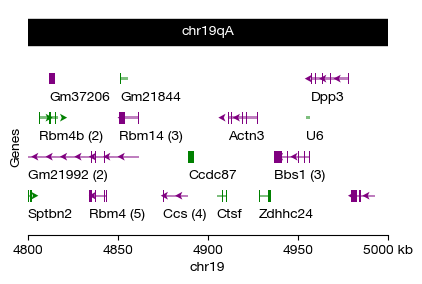
When zooming in to a narrower genomic window, individual gene structures become visible. Each gene model displays:

• Exons as wide blocks (coding exons filled, UTRs lighter)

• Introns as thin lines connecting exons

• Transcript arrows indicating the direction of transcription

The number in parentheses after each gene name indicates the count of annotated transcripts for that gene. Genes on the forward (sense) strand are shown in green, while genes on the reverse (antisense) strand are shown in purple. This color convention makes it easy to quickly identify transcriptional orientation and potential bidirectional transcription events.

Tip: A genomic window of ~200 kb or smaller is typically needed for individual exon structures to be resolvable. The exact threshold depends on the gene density of the region and the figure dimensions.

fig = genes(
    assembly = 'grcm39',
    chr = 'chr19',
    xfrom = 4800000,
    xto = 5000000,
    figsize = (4, 2.5)
)

Custom Multi-Track Compositions

The real power of the track system is in its composability — different track types can be freely stacked to create publication-ready multi-panel genomic region visualizations. The available track types are:

1. Gene track (gene_track): Annotated gene models (exons, introns, transcripts)

2. BED track (bed_track): Custom interval annotations (e.g., called peaks, blacklist regions)

3. Coverage tracks:

   • BAM coverage (coverage_track_from_bam): Read depth profile from aligned sequencing reads

   • BigWig coverage (coverage_track_from_bigwig): Pre-computed signal tracks (e.g., ChIP-seq, ATAC-seq)

4. Chromosome track (chromosome_track): Ideogram showing cytoband or assembly structure

The initialize_tracks() function creates a figure with the specified number of vertically stacked subplots (axes), all sharing the same genomic coordinate range. This ensures perfect alignment across tracks, enabling direct visual comparison of signals at the same genomic position.

Layout parameters:

• heights: Controls the relative height of each track (e.g., a chromosome track needs less vertical space than a gene track)

• figsize / dpi: Standard matplotlib figure dimensions

• The function returns the figure, axes list, tick positions, and coordinate bounds, which are then passed to individual track-drawing functions

Alignment principle: All tracks share identical xfrom / xto bounds. The xticks object is returned by initialize_tracks() and passed to coverage track functions to ensure matching x-axis label placement across all tracks.

# ============================================================
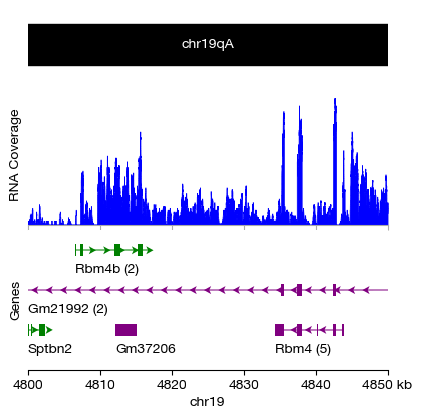
# Step 1: Initialize the multi-track figure layout
# ------------------------------------------------------------
# We create 3 vertically stacked tracks (subplots) sharing the
# same genomic window on chr19:4,800,000-4,850,000 (50 kb).
#
# heights = [0.2, 0.4, 0.4] — the chromosome ideogram is given
# less vertical space (0.2) compared to coverage and gene tracks (0.4 each)
# ============================================================
fig, axes, xticks, xticklabels, xfrom, xto = initialize_tracks(
    ntracks = 3,
    xfrom = 4800000, xto = 4850000, heights = [0.2, 0.4, 0.4],
    figsize = (4, 4), dpi = 100, sequence_name = 'chr19'
)

# ============================================================
# Step 2: Chromosome ideogram track (top)
# ------------------------------------------------------------
# Renders the cytoband pattern for the selected region.
# 'draw_label' is conditionally enabled only when the window
# is <= 25 Mb — for very zoomed-in views, drawing the full
# chromosome label clutters the figure.
# ============================================================
_, _ = chromosome_track(
    axes[0], xfrom, xto, chr = 'chr19', assembly = 'grcm39', color = 'cytobands',
    draw_label = (xfrom - xto) <= 25e6
)

# ============================================================
# Step 3: RNA-seq BAM coverage track (middle)
# ------------------------------------------------------------
# genome_track() configures shared track properties like axis labels.
# coverage_track_from_bam() reads the BAM file (requires a .bai index
# at the same path) and computes the per-base read depth profile
# over the [xfrom, xto) window. The signal is shown as a
# filled area plot.
#
# Note: Replace '/**/d1.sorted.bam' with the actual path to your
# indexed and sorted BAM file.
# ============================================================
_ = genome_track(axes[1], ylabel = 'RNA Coverage')
_ = coverage_track_from_bam(
    ax = axes[1], bam = '/**/d1.sorted.bam',
    xfrom = xfrom, xto = xto, chrm = 'chr19', xticks = xticks
)

# ============================================================
# Step 4: Gene annotation track (bottom)
# ------------------------------------------------------------
# gene_track() queries the reference annotation (GTF/GFF) stored
# in the exprmat database for the given assembly and renders
# gene models. It returns the gene data as a pandas DataFrame (gdf)
# for potential downstream use (e.g., identifying which genes
# overlap the region).
#
# show_gene_name=True displays gene symbols next to each model.
# ============================================================
_ = genome_track(axes[2], ylabel = 'Genes')
_, gdf = gene_track(
    axes[2], xfrom, xto, chr = 'chr19',
    assembly = 'grcm39', show_gene_name = True
)