Trajectory Inference#

For continuously varying phenotypic states, identifying marker genes using clustering methods is subjective and cannot provide definitive evidence for grouping, since most gene expression changes are dynamic. This situation is common in continuous cellular phenotypic transitions (developmental processes, polarization, slow reprogramming, etc.). Trajectory inference methods use a deliberately defined path on the kNN graph, assign cells to different positions along the path, and quantify gene expression changes based on these positional values.

Trajectory inference is entirely based on the kNN graph — if the kNN graph is inappropriate, the trajectory will be incorrect. Generally, UMAP accounts for local topological structure better than tSNE, while in some cases Diffusion Map is more suitable than UMAP (though this is not absolute). You need to choose a dimensionality reduction method that appropriately reflects the phenotypic topology in your dataset, and ensure that your data indeed captures intermediate cell populations. Sometimes, overly strong topological structure capture can introduce artificial false paths. Ideally, you should first observe in your dimensionality reduction plot that biologically relevant cells form connected graphs while unrelated cells form separate clusters. Sometimes, due to excessive missing data or other reasons, no reasonable path can be observed regardless of how you adjust the dimensionality reduction parameters. In such cases, trajectory inference is not suitable.

The start and end phenotypes for trajectory inference are entirely determined by the operator and require the operator’s prior knowledge. In the absence of experimentally validated prior knowledge, the direction of these trajectories may (and very likely will) be incorrect. Some computational methods such as RNA velocity and transcription factor entropy claim to infer trajectories, but their results do not always yield correct outcomes in practice.

[ ]:

%load_ext autoreload
%autoreload 2

[1]:

import exprmat as em
# set working directory
em.setwd('../../../data')
ver = em.version()

[i] exprmat 0.2.66 / exprmat-db 0.2.66
[i] os: posix (linux)  platform version: 6.8.0-90-generic
[i] loaded configuration from /home/data/yangz/.exprmatrc
[i] current working directory: /home/data/yangz/packages/exprmat/data
[i] current database directory: /home/data/yangz/packages/database (0.2.66)
[i] resident memory: 777.48 MiB
[i] virtual memory: 5.95 GiB

[2]:

expm = em.load_experiment('expm/scrna', load_samples = False, load_subset = 'mono-neutro')

[!] samples are not dumped in the experiment directory.

[3]:

print(expm)

annotated data of size 9754 × 19651
subset mono-neutro of size 9754 × 19651
contains modalities: rna

 modality [rna]
    obs : sample <cat> <c/sample> batch <cat> <c/batch> group <cat> <c> modality <cat> <c/modality>
          taxa <cat> <c/taxa> barcode <o> <o> ubc <o> <o> n.umi <f64> <i> n.genes <i64> <i>
          n.mito <f64> <f> n.ribo <f64> <f> pct.mito <f64> <f> pct.ribo <f64> <f>
          filter <bool> <bool> score.doublet <f64> <f> score.doublet.se <f64> <f>
          is.doublet <bool> <bool> qc <bool> <bool/qc> leiden <cat> <c> sc3.5 <cat> <c>
          sc3.10 <cat> <c> sc3.20 <cat> <c> sc3.30 <cat> <c> cell.type <cat> <c>
          kde.umap <f64> <f/kde> psbulk <cat>
    var : chr <cat> <c/chromosome> start <i64> <i> end <i64> <i> strand <cat> <c/strand> id <o> <o>
          subtype <cat> <c/gsubtype> gene <cat> <o/gene> tlen <f64> <i/tlen> cdslen <i64> <i/cdslen>
          assembly <cat> <c> uid <o> <o/ugene> vst.hvg <bool> <bool/hvg> vst.all.means <f64> <f>
          vst.all.vars <f64> <f> vst.all.vars.norm <f64> <f> vst.all.hvg.rank <f32> <f>
          vst.all.hvg <bool> <bool>
 layers : counts <f32> <i/counts> norm <f32> <f>
   obsm : cnmf.10 <df> <f/embedding/usage> harmony <arr:f32(35)> <f> knn <arr:i32(100)> <i/knni>
          knn.d <arr:f32(100)> <f/knnd> pca <arr:f64(35)> <f/embedding/pca>
          umap <arr:f32(2)> <f/embedding>
   varm : cnmf.10 <arr:f64(10)> <f/weights> cnmf.coef.10 <arr:f64(10)> <f/usage-coef>
          pca <arr:f64(35)> <f/weights>
   obsp : connectivities <csr:f32> <f/connectivity> distances <csr:f32> <f/distance>
    uns : cell.type.colors cell.type_colors cnmf <cnmf> cnmf.args <o>
          cnmf.density.10 <cnmf-density> cnmf.dist.10 <f/connectivity> cnmf.stats <cnmf-stats>
          commands <system> kde.umap <kde-stats> leiden <o> leiden.colors <o> markers <markers>
          neighbors <knn> pca <dict> sc3.10.colors <o> sc3.20.colors <o> sc3.30.colors <o>
          sc3.5.colors <o> slots <system> umap <o>

[*] samples not loaded from disk.

Diffmap dimensionality reduction#

Diffmap may capture topological structure information more sensitively than UMAP in some cases.

[4]:

expm.rna.diffmap(
    neighbors_key = 'neighbors', key_added = 'diffmap',
    n_comps = 5, sort = 'decrease', density_normalize = True,
    use_gpu = True
)

[5]:

expm.rna.knn(
    use_rep = 'diffmap',
    n_comps = None,
    n_neighbors = 30,
    knn = True,
    method = "umap",
    transformer = None,
    metric = "euclidean",
    metric_kwds = {},
    random_state = 42,
    key_added = 'nn30.diffmap',
    use_gpu = True
)

In our dataset, it performs similarly to UMAP, so we will still use 2D UMAP for trajectory inference. Notably, the first dimension of Diffmap almost never reflects developmental relationships — it shows the most prominent subpopulation information, unless your data contains only a single subpopulation.

[7]:

expm.rna.umap(
    min_dist = 0.30,
    spread = 0.6,
    n_components = 2,
    maxiter = None,
    alpha = 1,
    gamma = 1,
    negative_sample_rate = 5,
    init_pos = "spectral",
    random_state = 78,
    a = None,
    b = None,
    key_added = 'umap.diff',
    neighbors_key = "nn30.diffmap"
)

[16]:

fig = expm.rna.plot_embedding(
    basis = 'diffmap', embedding_dims = [1, 2], color = 'S100a8', annotate_style = 'text', legend = False,
    figsize = (3, 3), dpi = 100, ptsize = 4, contour_plot = False
)

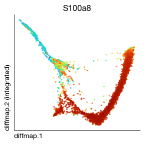
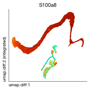
Running UMAP on the high dimensions of Diffmap to reduce to 2D is an interesting trick, but these trajectories may overfit and become distorted and ugly due to the nonlinear secondary transformation of UMAP.

[18]:

fig = expm.rna.plot_embedding(
    basis = 'umap.diff', color = 'S100a8', annotate_style = 'text', legend = False,
    figsize = (3, 3), dpi = 100, ptsize = 4, contour_plot = False
)

Principal curve inference#

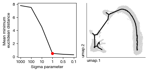
Next, we use an unsupervised method to infer possible trajectories from the structure of the dataset.

[19]:

expm.rna.principle_tree_explore_sigma(
    nodes = 200,
    use_rep = 'umap',
    ndims_rep = None,
    sigmas = [1000, 100, 10, 1, 0.5, 0.1],
    nsteps = 1,
    metric = "euclidean",
    seed = None,
    key_added = 'ppt'
)

[20]:

expm.rna.principle_tree(
    use_rep = 'umap',
    method = "ppt",
    init = None,
    ppt_sigma = 0.8, # test that
    ppt_lambda = 1,
    ppt_metric = "euclidean",
    ppt_nsteps = 60,
    ppt_err_cut = 5e-3,
    ppt_gpu_tpb = 16,
    device = "gpu",
    seed = 42,
    key_added = 'ppt',
)

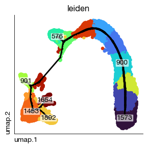
分岔点和终节点是轨迹中重要的关键阶段，你可以查看他们的编号，并考虑给他们一个人类可读的名字. 事实上，我们不推荐将不同谱系的细胞混合在一起进行轨迹推断，这可能会迷惑算法，并给出错误的路径

[21]:

fig = expm.rna.plot_graph(
    basis = 'umap',
    tips = True,
    forks = False,
    nodes = [900],
    rasterized = True,
    ax = None,
    trajectory_key = 'ppt',
    background_color = 'leiden',
    legend = False,
    annotate = False,
    ptsize = 20, alpha = 1,
    figsize = (3, 3),
    size_nodes = 2,
    cmap = 'turbo', default_color = 'lightgray'
)

Determining the trajectory direction#

The resulting tree-like trajectory has no direction — that is, at this step, the computer does not know which node in the graph corresponds to stem cells and which to terminally differentiated cells. You need to specify the starting point, and the algorithm will automatically identify the endpoints. In subsequent steps, you can also manually specify the start and end points to compute gene expression patterns.

Assessing absolute differentiation potential using CytoTrace scoring#

CytoTRACE2 is a neural network method trained on multiple human and mouse datasets for absolute differentiation potential prediction, and generalizes the predictions to other datasets. This method has only been validated in humans and mice, so caution is needed when applying it to other organisms.

[ ]:

expm.rna.cytotrace(
    key_counts = 'counts',
    key_gene = 'gene',
    taxa = 'mmu',
    batch_size = 20000,
    smooth_batch_size = 1000,
    disable_parallelization = False,
    max_cores = 30,
    seed = 42
)

[26]:

fig = expm.rna.plot_embedding(
    basis = 'umap', color = 'cytotrace.score', alpha = 0.5,
    figsize = (3, 3), dpi = 100, legend_col = 2, legend = False,
    ptsize = 6, annotate_style = 'text', contour_plot = False
)

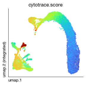
In fact, you should now analyze the granulocyte lineage and monocyte lineage separately to prevent the developmental trajectories from interfering with each other. But here we are only demonstrating the approach.

[27]:

expm.rna.principle_tree_root(trajectory_key = 'ppt', root = 576)

[i] node 576 selected as a root

[28]:

expm.rna.principle_tree_pseudotime(
    trajectory_key = 'ppt',
    seed = 42,
    cmap = 'category20b'
)

[i] projecting cells onto the principal graph

   ━━━━━━━━━━━━━━━━━━━━━━━━━━ mapping               2000 / 2000  (00:06 < 00:00)

[29]:

expm['rna'].obs[['ppt.pseudotime', 'ppt.seg', 'ppt.edge', 'ppt.milestones']]

[29]:

	ppt.pseudotime	ppt.seg	ppt.edge	ppt.milestones
distal:2	23.185281	7	1573\|1783	1573
distal:3	19.506181	7	705\|1276	1573
distal:4	12.648773	7	1728\|199	1573
distal:8	20.923024	7	1629\|353	1573
distal:9	13.109118	7	1853\|891	1573
...	...	...	...	...
normal:4657	8.907864	3	1651\|1047	195
normal:4658	14.847618	7	604\|1568	1573
normal:4660	18.582651	7	1412\|1691	1573
normal:4661	8.786800	7	717\|1271	1379
normal:4662	20.162801	7	930\|644	1573

9754 rows × 4 columns

The computer will calculate pseudotime based on the specified starting point, regardless of whether its direction is correct. As long as there is a computed order, you can reverse it later as needed when manually validating the path.

[30]:

fig = expm.rna.plot_principle_tree_segments(
    # trajectory plot
    basis = 'umap',
    color_seg = "milestones",
    trajectory_key = 'ppt',
    embedding_dims = [0, 1],
    annotate = True,

    # basis plot
    background_color = 'ppt.pseudotime', cmap = 'turbo', figsize = (4, 4),
    legend = False, default_color = 'lightgray',
    add_outline = True, outline_color = 'darkgray', alpha = 0.3, sort = True
)

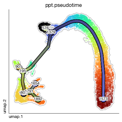
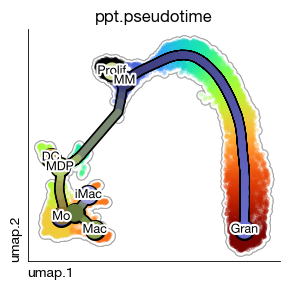
You can name some key nodes, and these names will be reflected in the plot.

[39]:

expm.rna.principle_tree_rename_milestones(
    trajectory_key = 'ppt',
    rename = {
        576: 'Prolif', 1379: 'MM', 1573: 'Gran',
        195: 'MDP', 901: 'DC', 1654: 'iMac', 1892: 'Mac', 1791: '', 807: '', 1453: 'Mo'
    }
)

[40]:

fig = expm.rna.plot_principle_tree_segments(
    # trajectory plot
    basis = 'umap',
    color_seg = "milestones",
    trajectory_key = 'ppt',
    embedding_dims = [0, 1],
    annotate = True,
    annotate_fontsize = 9,

    # basis plot
    background_color = 'ppt.pseudotime', cmap = 'turbo', figsize = (3, 3),
    legend = False, default_color = 'lightgray',
    add_outline = True, outline_color = 'darkgray', alpha = 0.3, sort = True
)

[ ]:

expm.save(save_samples = False)

Tracking gene expression patterns#

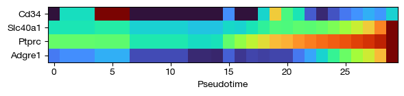
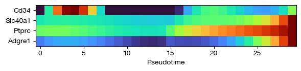
For a path you are interested in, you can discover which genes change significantly along that path and reveal their pattern of change.

This step involves regressing gene expression against pseudotime (in forward or reverse order, depending on your specified start and end points). If a gene is not constant with respect to pseudotime, it will be identified. To make the regression process more stable, we recommend imputing the sparse expression matrix. MAGIC is a recommended imputation algorithm based on graph diffusion. It runs reasonably well on datasets with fewer than 50k cells. However, its computational cost appears to increase nonlinearly with the number of cells.

[41]:

expm.rna.impute_magic(
    key_added = 'magic', solver = 'approximate', t = 'auto',
    random_state = 42, n_jobs = 60, n_pca = 30, knn = 15
)

[i] running MAGIC on 9754 cells and 19651 genes.
[!] you should remove empty genes before imputing with MAGIC.
Calculating PCA...
Calculated PCA in 3.56 seconds.
Calculating KNN search...
Calculated KNN search in 0.46 seconds.
Calculating affinities...
Calculated affinities in 1.22 seconds.
[i] automatically selected t = 6

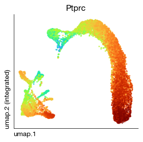
As you can see, the gene expression values have been smoothed.

[42]:

fig = expm.rna.plot_embedding(
    basis = 'umap', color = 'Ptprc', annotate_style = 'text', legend = False,
    figsize = (3, 3), dpi = 100, ptsize = 4, contour_plot = False, slot = 'magic'
)

Specify the node indices for source and destination, and the program will automatically find the shortest path between these two nodes in the trajectory graph. For example, node 576 is Prolif, and 1573 is the most differentiated Gran. Omitting source means using the previously specified root node as the starting point.

[43]:

expm.rna.principle_tree_trace(
    destination = 1573, source = 576,
    trajectory_key = 'ppt',
    lognorm = 'magic',
    binning = 15,
    statistic = 'mean',
    skip_sparsity = 40,
    order = 3,
    key_added = 'trace'
)

[!] there exists several shortest paths. returing a random one.

   ━━━━━━━━━━━━━━━━━━━━━━━━━━ regressing genes: 4  19651 / 19651 (00:17 < 00:00)
   ━━━━━━━━━━━━━━━━━━━━━━━━━━ regressing genes: 7  19651 / 19651 (00:17 < 00:00)

[44]:

expm['rna'].uns['trace'].obs[['chr', 'gene', 'leiden', 'p']]

[44]:

	chr	gene	leiden	p
rna:mmu:g8156	chr11	Gm12159	19	9.191839e-04
rna:mmu:g5189	chr10	Gja1	19	1.415043e-06
rna:mmu:g8568	chr11	Gm12246	19	9.243227e-07
rna:mmu:g58371	chr9	Hyls1	19	5.321373e-07
rna:mmu:g27362	chr18	Cdc25c	19	2.711096e-07
...	...	...	...	...
rna:mmu:g531	chr1	Kansl3	9	1.838810e-06
rna:mmu:g3254	chr1	Scyl3	9	4.672824e-07
rna:mmu:g23739	chr16	Gm32624	9	1.297662e-04
rna:mmu:g23754	chr16	Usp16	9	2.139328e-05
rna:mmu:g52942	chr7	Lrrc51	9	2.779056e-05

19651 rows × 4 columns

[45]:

fig = expm.rna.plot_principle_tree_trace(
    trace_key = 'trace',
    trajectory_key = 'ppt',
    values = 'expression',
    show_hvg_only = None,
    show_leiden_only = None,
    show_genes = ['Cd34', 'Ptprc', 'Adgre1', 'Slc40a1'],
    p_cutoff = 0.0001,
    cmap = 'turbo',
    figsize = (6, 1.5),
    show_gene_names = True
)

[46]:

fig = expm.rna.plot_principle_tree_trace(
    trace_key = 'trace',
    trajectory_key = 'ppt',
    values = 'fitted',
    show_hvg_only = None,
    show_leiden_only = None,
    show_genes = ['Cd34', 'Ptprc', 'Adgre1', 'Slc40a1'],
    p_cutoff = 0.0001,
    cmap = 'turbo',
    figsize = (6, 1.5),
    show_gene_names = True
)

[49]:

fig = expm.rna.plot_principle_tree_trace(
    trace_key = 'trace',
    trajectory_key = 'ppt',
    values = 'fitted',
    show_hvg_only = 'vst.hvg',
    show_leiden_only = [5, 21, 36],
    p_cutoff = 0.00001,
    cmap = 'turbo',
    figsize = (4, 20),
    show_gene_names = True
)

[51]:

expm.save()

[i] main dataset write to expm/scrna/subsets/mono-neutro.h5mu