Spliced Dynamics Inference#

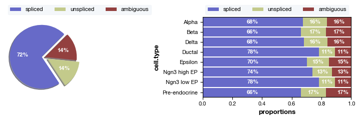
We can infer the gene expression using dynamics of the spliced and unspliced proportions of a gene’s transcripts.

[1]:

%load_ext autoreload
%autoreload 2

[2]:

import exprmat as em
# set working directory
em.setwd('../../../data')
ver = em.version()

[i] exprmat 0.2.66 / exprmat-db 0.2.66
[i] os: posix (linux)  platform version: 6.8.0-90-generic
[i] loaded configuration from /home/data/yangz/.exprmatrc
[i] current working directory: /home/data/yangz/packages/exprmat/data
[i] current database directory: /home/data/yangz/packages/database (0.2.66)
[i] resident memory: 777.88 MiB
[i] virtual memory: 5.95 GiB

[3]:

ver = em.version()

[i] exprmat 0.2.66 / exprmat-db 0.2.66
[i] os: posix (linux)  platform version: 6.8.0-90-generic
[i] loaded configuration from /home/data/yangz/.exprmatrc
[i] current working directory: /home/data/yangz/packages/exprmat/data
[i] current database directory: /home/data/yangz/packages/database (0.2.66)
[i] resident memory: 779.01 MiB
[i] virtual memory: 5.95 GiB

Initializing the splicing expression matrix from four count matrices#

The data below provides a standard 10X-format expression matrix, along with two additional matrices recording spliced and unspliced count matrices: We need the following file structure to automatically load the splicing matrices. These four MTX matrices and two TSV files are required.

[4]:

! tree -sh scrna/pancreas

[4.0K]  scrna/pancreas
├── [ 94K]  annotation.tsv
├── [ 15K]  barcodes.tsv.gz
├── [200K]  features.tsv.gz
├── [ 28M]  matrix.mtx.gz
├── [ 50M]  pancreas.h5ad
├── [9.3M]  spanning.mtx.gz
├── [ 28M]  spliced.mtx.gz
└── [9.3M]  unspliced.mtx.gz

1 directory, 8 files

[8]:

meta = em.metadata(
    # two samples from a murine tumor infiltrating cd8+ t cell dataset.
    locations    = [
        'scrna/pancreas',
        'scrna/pancreas',
    ],
    modality     = ['rna', 'rna/splicing'],
    default_taxa = ['mmu', 'mmu'],
    batches      = ['b-1', 'b-1'],
    names        = ['pancreas', 'pancreas'],
    groups       = ['pancreas', 'pancreas'],
)

[6]:

meta.dataframe

[6]:

	location	sample	batch	group	modality	taxa
0	scrna/pancreas	pancreas	b-1	pancreas	rna	mmu
1	scrna/pancreas	pancreas	b-1	pancreas	rna/splicing	mmu

[9]:

expm = em.experiment(meta, dump = 'expm/pancreas')

[i] reading sample pancreas [rna] ...
[i] 433 genes (out of 27998) not in the reference gene list.
[i] total 27565 genes mapped. 27543 unique genes.
[i] reading sample pancreas [rna/splicing] ...

[10]:

print(expm)

[!] dataset not integrated.
[*] composed of samples:
  pancreas   rna   mmu    batch b-1     of size 3696 × 27543

[ ]:

fig = expm.plot_rna_spliced_proportions(groupby = 'cell.type', figsize = (8, 2.5))

Quality control and visualization#

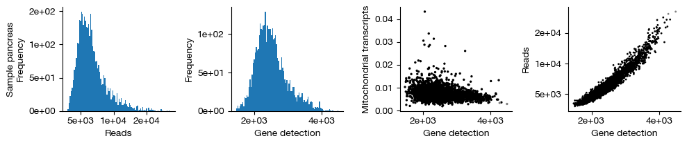
RNA dynamics inference generally requires a dataset that has already undergone marker gene selection, dimensionality reduction, clustering, and visualization. We first process the dataset using standard methods — see the Quality Control chapter for details.

[ ]:

expm.rna.qc(
    run_on_samples = True,
    mt_seqid = 'chrM',
    mt_percent = 0.15,
    ribo_genes = None,
    ribo_percent = None,
    outlier_mode = 'mads',
    outlier_n = 10,
    doublet_method = 'no',
    min_cells = 3,
    min_genes = 50,
)

   ━━━━━━━━━━━━━━━━━━━━━━━━━━ processing samples       1 / 1     (00:04 < 00:00)

[12]:

figs = expm.rna.plot_qc(run_on_samples = True)

[13]:

expm.merge(join = 'outer')

[14]:

expm.rna.log_normalize(
    key_norm = 'norm',
    key_lognorm = 'lognorm'
)

expm.rna.select_hvg(
    key_lognorm = 'X',
    method = 'vst',
    dest = 'vst',
    batch_key = 'batch',
    n_top_genes = 1500
)

[15]:

expm.rna.scale_pca(
    hvg = 'vst.hvg',
    key_lognorm = 'lognorm',
    key_scaled = 'scaled',
    key_added = 'pca', n_comps = 35,
    keep_sparse = False,
    random_state = 42,
    svd_solver = 'arpack'
)

[17]:

expm.rna.knn(
    use_rep = 'pca',
    n_comps = None,
    n_neighbors = 30,
    knn = True,
    method = "umap",
    transformer = None,
    metric = "cosine",
    metric_kwds = {},
    random_state = 42,
    key_added = 'neighbors'
)

expm.rna.leiden(
    resolution = 0.5,
    restrict_to = None,
    random_state = 42,
    key_added = 'leiden',
    adjacency = None,
    directed = None,
    use_weights = True,
    n_iterations = 2,
    partition_type = None,
    neighbors_key = None,
    obsp = None,
    flavor = 'igraph'
)

expm.rna.umap(
    min_dist = 0.5,
    spread = 1,
    n_components = 2,
    maxiter = None,
    alpha = 1,
    gamma = 1,
    negative_sample_rate = 5,
    init_pos = "spectral",
    random_state = 42,
    a = None, b = None,
    key_added = 'umap',
    neighbors_key = "neighbors"
)

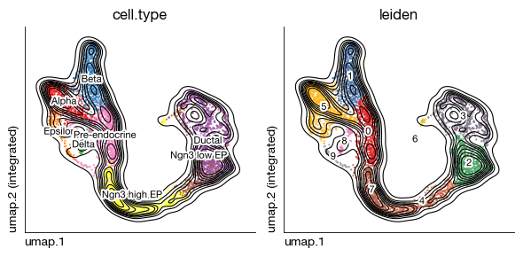
Now that we have obtained a dimensionality reduction representation and performed clustering, we can directly adopt the clustering information provided by the authors’ metadata. Note that the current dataset already contains three standard splicing matrices in the layers: spliced, unspliced, and ambiguous. These three matrices represent the count matrices for spliced transcripts, unspliced transcripts, and unclassified spanning reads, respectively.

[18]:

annots = em.pd.read_table('scrna/pancreas/annotation.tsv', index_col = 0)
expm['rna'].obs['cell.type'] = annots['clusters'].tolist()
expm['rna'].obs['cell.type'] = expm['rna'].obs['cell.type'].astype('category')
annots

[18]:

	clusters
index
AAACCTGAGAGGGATA	Pre-endocrine
AAACCTGAGCCTTGAT	Ductal
AAACCTGAGGCAATTA	Alpha
AAACCTGCATCATCCC	Ductal
AAACCTGGTAAGTGGC	Ngn3 high EP
...	...
TTTGTCAAGTGACATA	Pre-endocrine
TTTGTCAAGTGTGGCA	Ngn3 high EP
TTTGTCAGTTGTTTGG	Ductal
TTTGTCATCGAATGCT	Alpha
TTTGTCATCTGTTTGT	Epsilon

3696 rows × 1 columns

[19]:

fig = expm.rna.plot_multiple_embedding(
    basis = 'umap', features = ['cell.type', 'leiden'], ncols = 2, cmap = 'set1',
    figsize = (6, 3), dpi = 100, legend_col = 2, legend = False,
    ptsize = 2, annotate_style = 'text', annotate_fontsize = 8, contour_plot = True
)

[20]:

print(expm)

annotated data of size 3696 × 17584
integrated dataset of size 3696 × 17584
contains modalities: rna

 modality [rna]
    obs : sample <cat> <c/sample> batch <cat> <c/batch> group <cat> <c> modality <cat> <c/modality>
          taxa <cat> <c/taxa> barcode <o> <o> ubc <o> <o> n.umi <f64> <i> n.genes <i64> <i>
          n.mito <f64> <f> n.ribo <f64> <f> pct.mito <f64> <f> pct.ribo <f64> <f>
          filter <bool> <bool> score.doublet <f64> <f> score.doublet.se <f64> <f>
          is.doublet <bool> <bool> qc <bool> <bool/qc> leiden <cat> <c> cell.type <cat>
    var : chr <o> <c/chromosome> start <i64> <i> end <i64> <i> strand <o> <c/strand> id <o> <o>
          subtype <o> <c/gsubtype> gene <o> <o/gene> tlen <f64> <i/tlen> cdslen <i64> <i/cdslen>
          assembly <o> <c> uid <o> <o/ugene> vst.means <f64> <f> vst.vars <f64> <f>
          vst.vars.norm <f64> <f> vst.hvg.rank <f32> <f> vst.hvg <bool> <bool>
 layers : spliced <f64> <i/counts/spliced> unspliced <f64> <i/counts/unspliced>
          ambiguous <f64> <i/counts/ambiguous> norm <f32> <f/linear> lognorm <f32> <f/normal>
          counts <f32> <i/counts>
   obsm : pca <arr:f64(35)> <f/embedding/pca> knn <arr:i32(30)> <i/knni>
          knn.d <arr:f64(30)> <f/knnd> umap <arr:f32(2)> <f/embedding>
   varm : pca <arr:f64(35)> <f/weights>
   obsp : connectivities <csr:f32> <f/connectivity> distances <csr:f64> <f/distance>
    uns : slots <system> commands <system> pca <dict> neighbors <knn> leiden <o> umap
          cell.type.colors leiden.colors

[*] composed of samples:
  pancreas   rna   mmu    batch b-1     of size 3696 × 17584

RNA velocity inference#

The package already implements stochastic velocity inference.

[21]:

expm.rna.velocity(
    neighbor_key = 'neighbors', neighbor_connectivity = 'connectivities',
    n_neighbors = 30, hvg = 'vst.hvg', velocity_key = 'velocity',
    n_cpus = 100,
    kwargs_filter = {},
    kwargs_velocity = { 'mode': 'stochastic' },
    kwargs_velocity_graph = {},
    kwargs_terminal_state = {},
    kwargs_pseudotime = { 'save_diffmap': True }
)

[i] normalized count data: spliced, unspliced.
[i] computing moments based on connectivities
[i] computing velocities ...
[i] computing velocity graph (using 100/144 cores)

   ━━━━━━━━━━━━━━━━━━━━━━━━━━                       3696 / 3696  (00:09 < 00:00)

[i] computing terminal states ...
[i] identified 1 region of root cells and 1 region of end points .

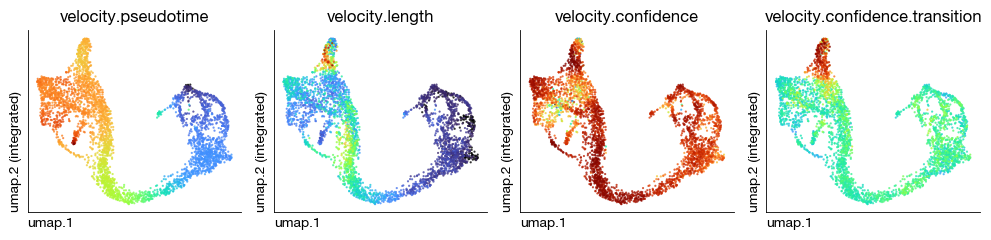
velocity.pseudotime, velocity.length, velocity.confidence, and velocity.confidence.transition — four velocity quality parameters — have been computed and automatically filled into the obs slot. We can now evaluate the reliability of the velocity estimates.

[22]:

print(expm)

annotated data of size 3696 × 17584
integrated dataset of size 3696 × 17584
contains modalities: rna

 modality [rna]
    obs : sample <cat> <c/sample> batch <cat> <c/batch> group <cat> <c> modality <cat> <c/modality>
          taxa <cat> <c/taxa> barcode <o> <o> ubc <o> <o> n.umi <f32> <i> n.genes <i64> <i>
          n.mito <f64> <f> n.ribo <f64> <f> pct.mito <f64> <f> pct.ribo <f64> <f>
          filter <cat> <bool> score.doublet <f64> <f> score.doublet.se <f64> <f>
          is.doublet <bool> <bool> qc <cat> <bool/qc> leiden <cat> <c> cell.type <cat>
          n.umi.unspliced <f64> <i> n.umi.spliced <f64> <i> velocity.self.transition <f32>
          root.cells <f64> <i> endpoints <f64> <i> velocity.pseudotime <f64> velocity.length <f32>
          velocity.confidence <f64> velocity.confidence.transition <f32>
    var : chr <cat> <c/chromosome> start <i64> <i> end <i64> <i> strand <cat> <c/strand> id <o> <o>
          subtype <cat> <c/gsubtype> gene <o> <o/gene> tlen <f64> <i/tlen> cdslen <i64> <i/cdslen>
          assembly <cat> <c> uid <o> <o/ugene> vst.means <f64> <f> vst.vars <f64> <f>
          vst.vars.norm <f64> <f> vst.hvg.rank <f32> <f> vst.hvg <bool> <bool> velocity.gamma <f32>
          velocity.qreg.ratio <f32> velocity.r2 <f64> velocity.genes <bool>
 layers : spliced <f64> <i/counts/spliced> unspliced <f64> <i/counts/unspliced>
          ambiguous <f64> <i/counts/ambiguous> norm <f32> <f/linear> lognorm <f32> <f/normal>
          counts <f32> <i/counts> spliced.counts <f64> <i/counts/spliced>
          unspliced.counts <f64> <i/counts/unspliced> ms <f32> <f/ms> mu <f32> <f/mu>
          velocity <f32> <f/vector> variance.velocity <f32>
   obsm : pca <arr:f64(35)> <f/embedding/pca> knn <arr:i32(30)> <i/knni>
          knn.d <arr:f64(30)> <f/knnd> umap <arr:f32(2)> <f/embedding> vdiff <arr:f64(10)> <f>
   varm : pca <arr:f64(35)> <f/weights>
   obsp : connectivities <csr:f32> <f/connectivity> distances <csr:f64> <f/distance>
    uns : slots <system> commands <system> pca <dict> neighbors <knn> leiden <o> umap
          cell.type.colors leiden.colors velocity.params velocity.graph velocity.graph.neg

[*] composed of samples:
  pancreas   rna   mmu    batch b-1     of size 3696 × 17584

[23]:

fig = expm.rna.plot_multiple_embedding(
    basis = 'umap', features = [
        'velocity.pseudotime', 'velocity.length', 'velocity.confidence', 'velocity.confidence.transition'
    ], ncols = 4, cmap = 'turbo',
    figsize = (10, 2.5), dpi = 100, legend_col = 2, legend = False,
    ptsize = 2, annotate_style = 'text', annotate_fontsize = 8, contour_plot = False
)

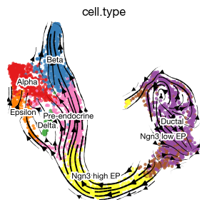
Given a 2D base embedding, we can project the high-dimensional velocity vectors onto UMAP for visualization.

[25]:

fig = expm.rna.plot_velocity_streamline(
    basis = 'umap', vkey = "velocity",
    neighbor_key = 'neighbors', frameon = False,
    color = 'cell.type', contour_plot = False, figsize = (3, 3), dpi = 100,
    density = 1.5, annotate_style = 'text', annotate_fontsize = 8
)

Saving the dataset#

Save the integrated dataset.

[26]:

expm.save(save_samples = False)

[i] main dataset write to expm/pancreas/integrated.h5mu