Single-cell ATAC-seq Analysis#
Single-cell ATAC-seq (scATAC-seq) presents unique computational challenges compared to bulk ATAC-seq or single-cell RNA-seq:
Extreme sparsity: scATAC-seq data is typically >95% sparse — most bins/peaks have zero counts in most cells, because each cell only contributes ~103-104 fragments covering <0.1% of the genome
High dimensionality: A typical analysis tiles the genome into millions of 500 bp bins, vs. ~20,000 genes in scRNA-seq
Binary nature: Unlike RNA counts which range from 0 to hundreds, ATAC-seq accessibility is essentially binary (a region is either accessible or not in a single cell)
These properties necessitate unsupervised clustering and dimensionality reduction as a first step before any biological interpretation. The standard workflow:
Tile the genome into equally-spaced bins (e.g., every 500 bp)
Construct a cell-by-bin count matrix
Select the most variable bins (feature selection)
Apply spectral embedding for dimensionality reduction
Cluster cells (Leiden algorithm)
Call peaks per cluster
Annotate cell types based on marker accessibility
This “bootstrap” approach is computationally intensive but essential for resolving cell-type-specific chromatin landscapes from sparse single-cell data.
[1]:
%load_ext autoreload
%autoreload 2
[2]:
import exprmat as em

em.setwd('../../../data')
ver = em.version()
[i] exprmat 0.2.66 / exprmat-db 0.2.66
[i] os: posix (linux)  platform version: 6.8.0-90-generic
[i] loaded configuration from /home/data/yangz/.exprmatrc
[i] current working directory: /home/data/yangz/packages/exprmat/data
[i] current database directory: /home/data/yangz/packages/database (0.2.66)
[i] resident memory: 777.56 MiB
[i] virtual memory: 5.95 GiB
[3]:
! tree -sh ./multiome
[4.0K]  ./multiome
├── [4.0K]  atac
│   └── [2.5G]  atac-pbmc-fragments.tsv.gz
└── [4.0K]  gex
    ├── [ 53K]  barcodes.tsv.gz
    ├── [2.7M]  features.tsv.gz
    └── [394M]  matrix.mtx.gz

3 directories, 4 files
[18]:
meta = em.metadata(
    locations    = [
        'multiome/atac/atac-pbmc-fragments.tsv.gz',
        'multiome/gex',
    ],
    modality     = ['atac', 'rna'],
    default_taxa = ['hsa/grch38', 'hsa/grch38'],
    batches      = ['b-1'] * 2,
    names        = ['atac', 'gex'],
    groups       = ['pbmc', 'pbmc'],
)
[19]:
meta.dataframe
[19]:
| location | sample | batch | group | modality | taxa | |
|---|---|---|---|---|---|---|
| 0 | multiome/atac/atac-pbmc-fragments.tsv.gz | atac | b-1 | pbmc | atac | hsa/grch38 |
| 1 | multiome/gex | gex | b-1 | pbmc | rna | hsa/grch38 |
[6]:
expm = em.experiment(meta, dump = 'expm/multiome')
[i] reading sample multiome [atac] ...
[i] reading sample multiome [rna] ...
[i] 939 genes (out of 36601) not in the reference gene list.
[i] total 35662 genes mapped. 35554 unique genes.
[7]:
expm.save()
[i] saving individual samples. (pass `save_samples = False` to skip)
   ━━━━━━━━━━━━━━━━━━━━━━━━━━ modality [atac]          1 / 1     (00:05 < 00:00)
   ━━━━━━━━━━━━━━━━━━━━━━━━━━ modality [rna]           1 / 1     (00:00 < 00:00)
Quality Control#
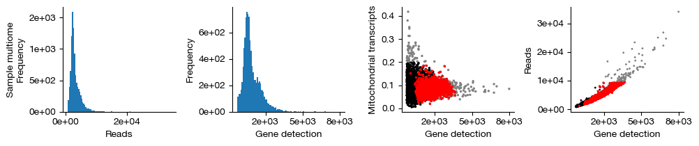
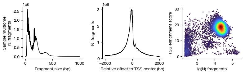
For multi-modal data with both scRNA-seq and scATAC-seq from the same cells (10x Multiome), we need to perform quality control separately for each modality before integration:
RNA QC includes:
Mitochondrial read fraction: High mt% (>20%) indicates dying/damaged cells
Ribosomal RNA fraction: Can indicate technical artifacts
Gene count / UMI count: Outlier detection using MAD (median absolute deviation)
Doublet detection: Using Scrublet to identify cell barcodes that contain two cells
ATAC QC includes:
Total fragment counts: Low counts = empty droplets, high counts = potential doublets
TSS enrichment score: Measures signal-to-noise around transcription start sites
Fraction of fragments in peaks (FRiP): Proportion of reads overlapping high-confidence peaks
Nucleosome signal ratio: Ratio of mono-nucleosomal to nucleosome-free fragments
[3]:
expm = em.load_experiment('expm/multiome')
━━━━━━━━━━━━━━━━━━━━━━━━━━ loading samples 2 / 2 (00:01 < 00:00)
[!] integrated mudata object is not generated.
[8]:
expm.atac.view('multiome')
annotated data of size 11431 × 0
    obs : n.fragments <ui64> pct.dup <f64> pct.mito <f64> barcode <o> ubc <o> sample <cat>
          batch <cat> group <cat> modality <cat> taxa <cat>
   obsm : paired <csr:ui32(3088286401)>
    uns : assembly.size assembly
[9]:
expm.rna.qc(
    run_on_samples = True,
    mt_seqid = 'chrM',
    mt_percent = 0.20,
    ribo_genes = None,
    ribo_percent = None,
    outlier_mode = 'mads',
    outlier_n = 10,
    doublet_method = 'scrublet',
    min_cells = 3,
    min_genes = 600
)
[i] found 13 mitochondrial genes (expected 13)
[i] found 106 ribosomal genes
quality controlling sample [multiome] ...
raw dataset contains 10970 cells, 28858 genes
[i] preprocessing observation count matrix ...
[i] simulating doublets ...
[i] embedding using pca ...
[i] calculating doublet scores ...
[i] detected doublet rate: 18.4 %
[i] estimated detectable doublet fraction: 98.8 %
[i] overall doublet rate: 18.7 %
filtered dataset contains 7828 cells, 24898 genes
[10]:
figs = expm.rna.plot_qc(run_on_samples = True)
[11]:
figs = expm.atac.plot_qc(run_on_samples = True)
[12]:
expm.rna.filter(run_on_samples = True)
expm.atac.filter_cells(
    run_on_samples = True,
    min_counts = 5000,
    min_tsse = 10,
    max_counts = 100000
)
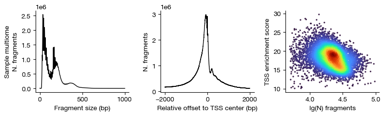
We retain only high-quality ATAC cells, characterized by:
High fragment count (≥5,000): Sufficient sequencing depth for reliable accessibility measurement
High TSS enrichment (≥10): Strong signal-to-noise ratio, indicating successful transposition at open chromatin
Moderate upper bound (≤100,000 fragments): Excluding potential doublets or artifacts
After filtering, we re-plot the QC metrics to verify that the retained cells meet quality standards. Note that the filtering thresholds should be adjusted based on data quality and sequencing depth — lower-depth datasets may require more lenient thresholds.
[14]:
figs = expm.atac.plot_qc(run_on_samples = True)
[15]:
print(expm)
[!] dataset not integrated.
[*] composed of samples:
  multiome   atac  hsa/grch38   batch b-1     of size 9868 × 0
  multiome   rna   hsa/grch38   batch b-1     of size 7828 × 24898
ATAC Fragment Matrix Construction and Clustering#
Unlike bulk ATAC-seq where peaks are called directly on pooled samples, single-cell ATAC-seq requires a different strategy. If we simply aggregate all fragments across all cells, we lose cell-type-specific information — the resulting “pseudo-bulk” peak set would be dominated by the most abundant cell types.
The challenge is a chicken-and-egg problem: We need cell-type-specific peak sets to understand chromatin landscapes, but we need to know the cell types first. To solve this, we perform unsupervised clustering using a genome-wide binning approach.
Key insight: Even though the cell-by-bin matrix is extremely sparse (~5% non-zero), it contains sufficient information to capture global chromatin accessibility patterns — cells of the same type will have similar patterns of open and closed bins across the genome.
First, we generate the cell-by-bin count matrix. By default, the genome is divided into 500 bp bins — a resolution that balances genomic coverage with computational feasibility. Each bin records the number of Tn5 cut sites (fragment endpoints) mapping to that interval for each cell.
Why 500 bp?
Too fine (e.g., 100 bp): Extremely high dimensionality (~30 million human genome bins), mostly zeros
Too coarse (e.g., 5 kb): Loses resolution for identifying regulatory elements
500 bp provides a good compromise, capturing local accessibility patterns while maintaining reasonable matrix dimensions
[16]:
expm.atac.make_bin_matrix(run_on_samples = True)
[17]:
expm.atac['multiome'].obs[['n.fragments', 'pct.dup', 'pct.mito', 'barcode', 'tsse']]
[17]:
| n.fragments | pct.dup | pct.mito | barcode | tsse | |
|---|---|---|---|---|---|
| multiome:1 | 22518 | 0.595487 | 0.0 | multiome:AAACGAAAGAGAGGTA-1 | 19.423177 |
| multiome:2 | 9019 | 0.499556 | 0.0 | multiome:AAACGAAAGCAGGAGG-1 | 22.519364 |
| multiome:3 | 28148 | 0.524141 | 0.0 | multiome:AAACGAAAGGAAGAAC-1 | 17.890528 |
| multiome:4 | 29126 | 0.570552 | 0.0 | multiome:AAACGAAAGTCGACCC-1 | 19.469426 |
| multiome:5 | 13124 | 0.562606 | 0.0 | multiome:AAACGAACAAGCACTT-1 | 22.730108 |
| ... | ... | ... | ... | ... | ... |
| multiome:11427 | 42232 | 0.446624 | 0.0 | multiome:TTTGTGTTCTATACCT-1 | 15.579201 |
| multiome:11428 | 19064 | 0.511880 | 0.0 | multiome:TTTGTGTTCTATCTCA-1 | 18.225700 |
| multiome:11429 | 24653 | 0.545801 | 0.0 | multiome:TTTGTGTTCTCTATTG-1 | 18.913518 |
| multiome:11430 | 25610 | 0.485908 | 0.0 | multiome:TTTGTGTTCTGATCTT-1 | 15.025295 |
| multiome:11431 | 24949 | 0.513513 | 0.0 | multiome:TTTGTGTTCTTACTCA-1 | 19.920115 |
9868 rows × 5 columns
We can see that the human genome (GRCh38) is divided into approximately 6.06 million 500 bp bins. This is the initial feature space — each column in .var represents one genomic bin with its chromosome, start, and end coordinates.
Similar to highly-variable gene selection in scRNA-seq, we need to filter out the overwhelming majority of bins that contain only zeros or near-zero counts. We select 250,000 highly-variable chromatin bins (HVCs) — bins that show the most variance across cells.
Why 250K and not 1K-2K (like scRNA-seq)?
scRNA-seq typically selects 1,000-2,000 highly variable genes (HVGs) from ~20,000 total genes
For scATAC-seq, the feature space is ~6 million bins, and the information per feature is much sparser
We need more features to capture the complex, combinatorial patterns of chromatin accessibility
250,000 HVCs (~4% of total bins) provides sufficient signal for robust cell clustering while being computationally tractable
Selection criterion: Bins are ranked by a dispersion-based metric (variance/mean ratio), accounting for the relationship between mean accessibility and variance.
[18]:
expm.atac.select_features(
    run_on_samples = True,
    n_features = int(25e4)
)
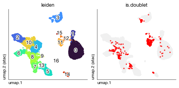
Using an adapted Scrublet method, we can efficiently detect doublets from scATAC-seq data. The original Scrublet was designed for scRNA-seq; the ATAC-adapted version:
Simulates “neighbor” doublets by combining pairs of observed cell profiles
Computes a doublet score for each cell based on the density of simulated doublets in its local neighborhood
Thresholds the scores to classify cells as putative doublets
This step is important because doublets in scATAC-seq can create spurious “clusters” that mix accessibility signals from different cell types.
[19]:
expm.atac.scrublet(
    run_on_samples = True,
    scrublet_init_args = { 'random_state': 42 },
    scrublet_args = {}
)
[i] preprocessing observation count matrix ...
[i] simulating doublets ...
[i] embedding using spectrum ...
[i] calculating doublet scores ...
[i] detected doublet rate: 6.1 %
[i] estimated detectable doublet fraction: 72.0 %
[i] overall doublet rate: 8.4 %
[ ]:
expm.save()
[i] main dataset write to expm/multiome/integrated.h5mu
[i] saving individual samples. (pass `save_samples = False` to skip)
   ━━━━━━━━━━━━━━━━━━━━━━━━━━ modality [atac]          1 / 1     (00:42 < 00:00)
   ━━━━━━━━━━━━━━━━━━━━━━━━━━ modality [rna]           1 / 1     (00:00 < 00:00)
Dimensionality Reduction and Clustering#
We use Spectral Embedding for unsupervised dimensionality reduction of the highly-variable chromatin bins. Spectral embedding is particularly well-suited for scATAC-seq data because:
It captures non-linear relationships in the data better than PCA
It constructs a similarity graph between cells using cosine distance, which is robust for sparse binary data
The eigenvectors of the graph Laplacian provide a low-dimensional representation that preserves the global data structure
The workflow:
Spectral decomposition: Compute the top 30 spectral components from the cell-by-HVC matrix
KNN graph: Build a 30-nearest-neighbor graph in the spectral embedding space
UMAP: Compute a 2D visualization from the neighbor graph
Leiden clustering: Apply the Leiden algorithm (an improvement over Louvain) at resolution 0.5 to identify cell communities
Leiden algorithm is a graph-based community detection method that:
Optimizes modularity to partition the cell similarity graph
Resolution parameter controls coarseness (higher = more clusters)
Resolution 0.5 is a conservative choice suitable for initial exploratory analysis
[3]:
expm = em.load_experiment('expm/multiome')
━━━━━━━━━━━━━━━━━━━━━━━━━━ loading samples 2 / 2 (00:15 < 00:00)
[!] integrated mudata object is not generated.
[5]:
expm.atac.view('atac')
annotated data of size 9868 × 6176584
    obs : n.fragments <ui64> <i> pct.dup <f64> <f> pct.mito <f64> <f> barcode <o> <o> ubc <o> <o>
          sample <cat> <c/sample> batch <cat> <c/batch> group <cat> <c> modality <cat> <c/modality>
          taxa <cat> <c/taxa> tsse <f64> <f/tsse> n.umi <ui64> <i> score.doublet <f64> <f>
          score.doublet.se <f64> <f> is.doublet <bool> <bool>
    var : chr <cat> <c/chromosome> start <cat> <i> end <cat> <i> location <o> <o/location>
          unique <o> <o> count <f64> selected <bool> <bool>
   obsm : paired <csr:ui32(3088286401)> <fragments> spectral <arr:f64(30)>
    uns : assembly <assembly> assembly.size <asm-size> frag.sizes <frag-size>
          pct.tss.overlap <tss-overlap> scrublet <scrublet> simulated <scrublet-simulated>
          tss.profile <tss-profile> tsse <overall-tsse>
[6]:
expm.atac.select_features(
    run_on_samples = True,
    n_features = int(25e4)
)
[7]:
expm.atac.spectral(
    run_on_samples = True,
    n_comps = 30,
    features = "selected",
    random_state = 0,
    sample_size = None,
    sample_method = "random",
    chunk_size = 20000,
    distance_metric = "cosine",
    weighted_by_sd = True,
    feature_weights = None,
    key_added = 'spectral'
)
[8]:
expm.atac.knn(
    run_on_samples = True,
    use_rep = 'spectral',
    n_comps = None,
    n_neighbors = 30,
    knn = True,
    method = "umap",
    transformer = None,
    metric = "cosine",
    metric_kwds = {},
    random_state = 0,
    key_added = 'neighbors',
    n_jobs = -1,
    use_gpu = True
)
[9]:
expm.atac.umap(
    run_on_samples = True,
    n_components = 2,
    neighbors_key = 'neighbors'
)
[10]:
expm.atac.leiden(
    run_on_samples = True,
    resolution = 0.5
)
[11]:
fig = expm.atac.plot_multiple_embedding(
    run_on_samples = True,
    basis = 'umap', features = ['leiden', 'is.doublet'], ncols = 2, figsize = (6, 3),
    legend = False, annotate = True, annotate_style = 'text'
)
Inferring Gene Activity from ATAC-seq#
One of the most useful outputs of scATAC-seq analysis is an inferred gene activity matrix (automatically append as a rna modality sample of the same name). This bridges the gap between chromatin accessibility and gene expression by estimating transcriptional activity from promoter accessibility.
Method:
For each gene, define its regulatory window (typically ±2 kb around the transcription start site)
Sum the ATAC-seq signal (Tn5 cut sites) within that window
This produces a gene-by-cell matrix analogous to scRNA-seq expression data
Use cases:
Cross-modal integration: Align ATAC-seq cells with RNA-seq cells using shared gene activity features
Cell type annotation: Use known marker genes to label clusters (e.g., CD3D for T cells)
Comparative analysis: Directly compare chromatin-based “expression” with RNA expression
Important caveat: The gene activity matrix is:
Very sparse (more so than RNA)
Noisy (promoter accessibility is an imperfect proxy for expression)
Biased toward highly expressed / housekeeping genes
[13]:
expm.atac.infer_gene_activity_fragments(
    run_on_samples = True,
)
[i] created subset [atac] from sample [atac]
[14]:
print(expm)
[!] dataset not integrated.
[*] composed of samples:
  atac    atac  hsa/grch38   batch b-1     of size 9868 × 6176584
  gex     rna   hsa/grch38   batch b-1     of size 7828 × 24898
  atac    rna   hsa/grch38   batch b-1     of size 9868 × 75716
[16]:
expm.rna.view('atac')
annotated data of size 9868 × 75716
    obs : n.fragments <ui64> <i> pct.dup <f64> <f> pct.mito <f64> <f> barcode <o> <o> ubc <o> <o>
          sample <cat> <c/sample> batch <cat> <c/batch> group <cat> <c> modality <cat> <c/modality>
          taxa <cat> <c/taxa> tsse <f64> <f/tsse> n.umi <ui64> <i> score.doublet <f64> <f>
          score.doublet.se <f64> <f> is.doublet <bool> <bool> leiden <cat> <c>
    var : chr <o> <c/chromosome> start <i64> <i> end <i64> <i> strand <o> <c/strand> id <o> <o>
          subtype <o> <c/gsubtype> gene <o> <o/gene> tlen <f64> <i/tlen> cdslen <i64> <i/cdslen>
          assembly <o> <c> uid <o> <o/ugene>
   obsm : spectral <arr:f64(29)> <f/embedding> knn <arr:i32(30)> <i> knn.d <arr:f32(30)> <f>
          umap <arr:f32(2)> <f>
    uns : assembly <assembly> assembly.size <asm-size>
[18]:
expm.rna.view('gex')
annotated data of size 7828 × 24898
    obs : sample <cat> <c/sample> batch <cat> <c/batch> group <cat> <c> modality <cat> <c/modality>
          taxa <cat> <c/taxa> barcode <o> <o> ubc <o> <o> n.umi <f64> <i> n.genes <i64> <i>
          n.mito <f64> <f> n.ribo <f64> <f> pct.mito <f64> <f> pct.ribo <f64> <f>
          filter <bool> <bool> score.doublet <f64> <f> score.doublet.se <f64> <f>
          is.doublet <bool> <bool> qc <bool> <bool/qc>
    var : chr <cat> <c/chromosome> start <i64> <i> end <i64> <i> strand <cat> <c/strand> id <o> <o>
          subtype <cat> <c/gsubtype> gene <cat> <o/gene> tlen <f64> <i/tlen> cdslen <i64> <i/cdslen>
          assembly <cat> <c> uid <o> <o/ugene> n.umi <f64> <i> n.cells <i64> <i> qc <bool> <bool/qc>
    uns : scrublet <scrublet>
[19]:
expm.rna['atac'].obs[['barcode', 'leiden']]
[19]:
| barcode | leiden | |
|---|---|---|
| multiome:1 | multiome:AAACGAAAGAGAGGTA-1 | 0 |
| multiome:2 | multiome:AAACGAAAGCAGGAGG-1 | 2 |
| multiome:3 | multiome:AAACGAAAGGAAGAAC-1 | 3 |
| multiome:4 | multiome:AAACGAAAGTCGACCC-1 | 4 |
| multiome:5 | multiome:AAACGAACAAGCACTT-1 | 4 |
| ... | ... | ... |
| multiome:11427 | multiome:TTTGTGTTCTATACCT-1 | 0 |
| multiome:11428 | multiome:TTTGTGTTCTATCTCA-1 | 5 |
| multiome:11429 | multiome:TTTGTGTTCTCTATTG-1 | 7 |
| multiome:11430 | multiome:TTTGTGTTCTGATCTT-1 | 0 |
| multiome:11431 | multiome:TTTGTGTTCTTACTCA-1 | 9 |
9868 rows × 2 columns
[20]:
expm.rna['atac'].var[['chr', 'strand', 'start', 'end', 'gene', 'assembly']]
[20]:
| chr | strand | start | end | gene | assembly | |
|---|---|---|---|---|---|---|
| rna:hsa:g78927 | chrY | - | 57212184 | 57214397 | DDX11L16 | grch38 |
| rna:hsa:g63727 | chr1 | + | 12010 | 13670 | DDX11L1 | grch38 |
| rna:hsa:g63728 | chr1 | - | 14696 | 24886 | WASH7P | grch38 |
| rna:hsa:g3 | chr1 | - | 17369 | 17436 | MIR6859-1 | grch38 |
| rna:hsa:g4 | chr1 | + | 28589 | 31109 | MIR1302-2HG | grch38 |
| ... | ... | ... | ... | ... | ... | ... |
| rna:hsa:g78919 | chrY | - | 26586642 | 26591601 | SLC25A15P1 | grch38 |
| rna:hsa:g78920 | chrY | - | 26594851 | 26634652 | PARP4P1 | grch38 |
| rna:hsa:g78921 | chrY | - | 26626520 | 26627159 | CCNQP2 | grch38 |
| rna:hsa:g78922 | chrY | + | 56855244 | 56855488 | CTBP2P1 | grch38 |
| rna:hsa:g63718 | chrY | + | 56881849 | 56882115 | ENSG00000305394 | grch38 |
75716 rows × 6 columns
[21]:
fig = expm.rna.plot_embedding(
    run_on_samples = ['atac'],
    basis = 'umap', color = 'GZMB', figsize = (3, 3)
)
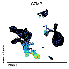
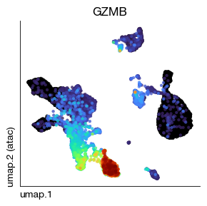
To address the sparsity of the gene activity matrix, we apply MAGIC (Markov Affinity-based Graph Imputation of Cells) smoothing. MAGIC is a diffusion-based imputation method that:
Constructs a graph where cells are connected based on accessibility profile similarity
Uses a Markov transition matrix to diffuse information across the graph
Smooths gene activity values by sharing information between similar cells
The
tparameter controls the diffusion strength —t='auto'automatically selects an appropriate number of diffusion steps
Parameters:
solver='approximate': Uses an approximate (faster) diffusion solvert='auto': Automatically determines the number of diffusion stepsn_pca=30: Uses 30 PCA components for initial distance computationknn=15: 15-nearest-neighbor graph for defining cell-cell affinities
Before vs. after: Compare the GZMB (Granzyme B, a cytotoxic marker) UMAP plots before and after MAGIC imputation. The smoothed version should show clearer, more continuous expression patterns.
[24]:
expm.rna.impute_magic(
    run_on_samples = ['atac'],
    layer = 'X', # of raw counts
    key_added = 'magic', solver = 'approximate', t = 'auto',
    random_state = 42, n_jobs = 1, n_pca = 30, knn = 15
)
[i] running MAGIC on 9868 cells and 75716 genes.
Calculating PCA...
Calculated PCA in 28.49 seconds.
Calculating KNN search...
Calculated KNN search in 0.42 seconds.
Calculating affinities...
Calculated affinities in 0.66 seconds.
[i] automatically selected t = 5
[25]:
fig = expm.rna.plot_embedding(
    run_on_samples = ['atac'],
    slot = 'magic',
    basis = 'umap', color = 'GZMB', figsize = (3, 3)
)
Merge dataset#
[47]:
expm.merge()
[48]:
print(expm)
annotated data of size 17696 × 75855
annotated data of size 9868 × 6176584
integrated dataset of size 17696 × 6252439
contains modalities: rna, atac

 modality [rna]
    obs : sample <cat> <c/sample> batch <cat> <c/batch> group <cat> <c> modality <cat> <c/modality>
          taxa <cat> <c/taxa> barcode <o> <o> ubc <o> <o> n.umi <f64> <i> n.genes <f64> <i>
          n.mito <f64> <f> n.ribo <f64> <f> pct.mito <f64> <f> pct.ribo <f64> <f>
          filter <boolean> <bool> score.doublet <f64> <f> score.doublet.se <f64> <f>
          is.doublet <bool> <bool> qc <boolean> <bool/qc> n.fragments <f64> <f> pct.dup <f64> <f>
          tsse <f64> <f> leiden <cat> <o>
    var : chr <o> <c/chromosome> start <i64> <i> end <i64> <i> strand <o> <c/strand> id <o> <o>
          subtype <o> <c/gsubtype> gene <o> <o/gene> tlen <f64> <i/tlen> cdslen <i64> <i/cdslen>
          assembly <o> <c> uid <o> <o/ugene>
    uns : slots <system>

 modality [atac]
    obs : n.fragments <ui64> <i> pct.dup <f64> <f> pct.mito <f64> <f> barcode <o> <o> ubc <o> <o>
          sample <cat> <c/sample> batch <cat> <c/batch> group <cat> <c> modality <cat> <c/modality>
          taxa <cat> <c/taxa> tsse <f64> <f/tsse> n.umi <ui64> <i> score.doublet <f64> <f>
          score.doublet.se <f64> <f> is.doublet <bool> <bool> leiden <cat> <c>
    var : chr <cat> <c/chromosome> start <cat> <i> end <cat> <i> location <o> <o/location>
          unique <o> <o>
   obsm : paired <csr:ui32(3088286401)> <fragments>
    uns : assembly <assembly> assembly.size <asm-size> slots <system>

[*] composed of samples:
  atac    atac  hsa/grch38   batch b-1     of size 9868 × 6176584
  gex     rna   hsa/grch38   batch b-1     of size 7828 × 24898
  atac    rna   hsa/grch38   batch b-1     of size 9868 × 75716
Cluster-Specific Peak Calling#
Now that we have identified cell clusters (from the unsupervised Leiden clustering), we can aggregate fragments within each cluster and call peaks separately per cluster. This is analogous to the group-level peak calling in bulk ATAC-seq, but here the “groups” are data-driven cell populations.
Why per-cluster peak calling?
Different cell types have distinct open chromatin landscapes
A peak present only in one cell type would be diluted or missed in a pooled analysis
Per-cluster peaks enable identification of cell-type-specific regulatory elements
[49]:
expm.atac.call_peaks_fragments(
    # call peaks from fragments
    groupby = 'leiden',
    qvalue = 0.05,
    call_broad_peaks = False,
    broad_cutoff = 0.1,
    replicate = None,
    replicate_qvalue = None,
    max_frag_size = 180,  # only call nucleosome-free fragments
    selections = None,
    nolambda = False,
    shift = -100,
    extsize = 200,
    min_len = None,
    blacklist = None,
    # directly call groups of peaks
    key_added = 'peaks.leiden',
    inplace = True,
    n_jobs = 30
)
[i] exporting fragments ...
[i] calling peaks ...
For example, we can inspect the peaks called for Leiden cluster 0. The output shows the peak coordinates (chromosome, start, end), summit position, and significance metrics (q-value, fold enrichment). Each cluster’s peaks are stored in a dedicated entry under .uns['peaks.leiden'].
[50]:
expm['atac'].uns['peaks.leiden']['0']
[50]:
| chr | start | end | peak | score | strand | fc | p | q | summit | |
|---|---|---|---|---|---|---|---|---|---|---|
| 0 | chr1 | 180730 | 180986 | . | 81 | . | 4.288069 | 10.100930 | 8.183347 | 129 |
| 1 | chr1 | 191357 | 191634 | . | 127 | . | 5.317205 | 14.739340 | 12.765400 | 141 |
| 2 | chr1 | 191723 | 191974 | . | 233 | . | 7.375478 | 25.418261 | 23.355879 | 125 |
| 3 | chr1 | 267865 | 268140 | . | 1000 | . | 19.553593 | 110.513199 | 108.136642 | 136 |
| 4 | chr1 | 271171 | 271442 | . | 410 | . | 10.166667 | 43.203339 | 41.043182 | 133 |
| ... | ... | ... | ... | ... | ... | ... | ... | ... | ... | ... |
| 133923 | chrY | 21440574 | 21440925 | . | 880 | . | 16.980751 | 90.334290 | 88.009842 | 160 |
| 133924 | chrY | 21481578 | 21481878 | . | 396 | . | 10.119842 | 41.849751 | 39.695633 | 153 |
| 133925 | chrY | 21650560 | 21650859 | . | 119 | . | 5.145682 | 13.929480 | 11.964249 | 132 |
| 133926 | chrY | 56838962 | 56839229 | . | 54 | . | 3.601978 | 7.336670 | 5.464052 | 123 |
| 133927 | chrY | 56839508 | 56839908 | . | 20 | . | 2.572841 | 3.803030 | 2.017889 | 94 |
133928 rows × 10 columns
After calling peaks per cluster, we merge them into a consensus peak set across all clusters and construct the peak-by-cell count matrix. The merging step uses the SnapATAC algorithm to produce a unified set of peak intervals, which are then used for counting (similar to the bulk ATAC-seq workflow).
[ ]:
expm.atac.merge_peaks_fragments(
    key_added = 'peaks.merged',
    key_groups = 'peaks.leiden',
    flavor = 'snapatac'
)
[52]:
print(expm)
annotated data of size 17696 × 75855
annotated data of size 9868 × 6176584
integrated dataset of size 17696 × 6252439
contains modalities: rna, atac

 modality [rna]
    obs : sample <cat> <c/sample> batch <cat> <c/batch> group <cat> <c> modality <cat> <c/modality>
          taxa <cat> <c/taxa> barcode <o> <o> ubc <o> <o> n.umi <f64> <i> n.genes <f64> <i>
          n.mito <f64> <f> n.ribo <f64> <f> pct.mito <f64> <f> pct.ribo <f64> <f>
          filter <boolean> <bool> score.doublet <f64> <f> score.doublet.se <f64> <f>
          is.doublet <bool> <bool> qc <boolean> <bool/qc> n.fragments <f64> <f> pct.dup <f64> <f>
          tsse <f64> <f> leiden <cat> <o>
    var : chr <o> <c/chromosome> start <i64> <i> end <i64> <i> strand <o> <c/strand> id <o> <o>
          subtype <o> <c/gsubtype> gene <o> <o/gene> tlen <f64> <i/tlen> cdslen <i64> <i/cdslen>
          assembly <o> <c> uid <o> <o/ugene>
    uns : slots <system>

 modality [atac]
    obs : n.fragments <ui64> <i> pct.dup <f64> <f> pct.mito <f64> <f> barcode <o> <o> ubc <o> <o>
          sample <cat> <c/sample> batch <cat> <c/batch> group <cat> <c> modality <cat> <c/modality>
          taxa <cat> <c/taxa> tsse <f64> <f/tsse> n.umi <ui64> <i> score.doublet <f64> <f>
          score.doublet.se <f64> <f> is.doublet <bool> <bool> leiden <cat> <c>
    var : chr <cat> <c/chromosome> start <cat> <i> end <cat> <i> location <o> <o/location>
          unique <o> <o>
   obsm : paired <csr:ui32(3088286401)> <fragments>
    uns : assembly <assembly> assembly.size <asm-size> slots <system>
          peaks.leiden <dict/peaks/grouped-peaks> commands <system>
          peaks.merged <dict/peaks/merged-peaks>

[*] composed of samples:
  atac    atac  hsa/grch38   batch b-1     of size 9868 × 6176584
  gex     rna   hsa/grch38   batch b-1     of size 7828 × 24898
  atac    rna   hsa/grch38   batch b-1     of size 9868 × 75716
[59]:
expm.atac.make_peak_matrix_fragments(
    chunk_size = 500,
    min_frag_size = None,
    max_frag_size = 180,
    counting_strategy = 'paired-insertion',
    value_type = 'target',
    summary_type = 'sum'
)
[i] created subset [integrated] from sample [integrated]
[!] you are mutating the integrated mudata object via a dataset generator.
[!] this is not recommended, since the existing modality will be replaced if there is one.
[60]:
print(expm)
annotated data of size 17696 × 75855
annotated data of size 9868 × 6176584
annotated data of size 9868 × 215677
integrated dataset of size 17696 × 6468116
contains modalities: rna, atac, atac-peak

 modality [rna]
    obs : sample <cat> <c/sample> batch <cat> <c/batch> group <cat> <c> modality <cat> <c/modality>
          taxa <cat> <c/taxa> barcode <o> <o> ubc <cat> <o> n.umi <f64> <i> n.genes <f64> <i>
          n.mito <f64> <f> n.ribo <f64> <f> pct.mito <f64> <f> pct.ribo <f64> <f>
          filter <boolean> <bool> score.doublet <f64> <f> score.doublet.se <f64> <f>
          is.doublet <bool> <bool> qc <boolean> <bool/qc> n.fragments <f64> <f> pct.dup <f64> <f>
          tsse <f64> <f> leiden <cat> <o>
    var : chr <cat> <c/chromosome> start <i64> <i> end <i64> <i> strand <cat> <c/strand> id <o> <o>
          subtype <cat> <c/gsubtype> gene <cat> <o/gene> tlen <f64> <i/tlen> cdslen <i64> <i/cdslen>
          assembly <cat> <c> uid <o> <o/ugene>
    uns : slots <system>

 modality [atac]
    obs : n.fragments <ui64> <i> pct.dup <f64> <f> pct.mito <f64> <f> barcode <o> <o> ubc <o> <o>
          sample <cat> <c/sample> batch <cat> <c/batch> group <cat> <c> modality <cat> <c/modality>
          taxa <cat> <c/taxa> tsse <f64> <f/tsse> n.umi <ui64> <i> score.doublet <f64> <f>
          score.doublet.se <f64> <f> is.doublet <bool> <bool> leiden <cat> <c>
    var : chr <cat> <c/chromosome> start <cat> <i> end <cat> <i> location <o> <o/location>
          unique <o> <o>
   obsm : paired <csr:ui32(3088286401)> <fragments>
    uns : assembly <assembly> assembly.size <asm-size> slots <system>
          peaks.leiden <dict/peaks/grouped-peaks> commands <system>
          peaks.merged <dict/peaks/merged-peaks>

 modality [atac-peak]
    obs : n.fragments <ui64> <i> pct.dup <f64> <f> pct.mito <f64> <f> barcode <o> <o> ubc <o> <o>
          sample <cat> <c/sample> batch <cat> <c/batch> group <cat> <c> modality <cat> <c/modality>
          taxa <cat> <c/taxa> tsse <f64> <f/tsse> n.umi <ui64> <i> score.doublet <f64> <f>
          score.doublet.se <f64> <f> is.doublet <bool> <bool> leiden <cat> <c>
    var : 12 <bool> <bool> 15 <bool> <bool> 6 <bool> <bool> 11 <bool> <bool> 8 <bool> <bool>
          9 <bool> <bool> 2 <bool> <bool> 7 <bool> <bool> 5 <bool> <bool> 3 <bool> <bool>
          16 <bool> <bool> 14 <bool> <bool> 0 <bool> <bool> 13 <bool> <bool> 1 <bool> <bool>
          10 <bool> <bool> 4 <bool> <bool> chr <o> <c/chromosome> start <i64> <i> end <i64> <i>
          strand <o> <o/strand> summit <i64> <i>
    uns : assembly <assembly> assembly.size <asm-size> slots <system>

[*] composed of samples:
  atac    atac  hsa/grch38   batch b-1     of size 9868 × 6176584
  gex     rna   hsa/grch38   batch b-1     of size 7828 × 24898
  atac    rna   hsa/grch38   batch b-1     of size 9868 × 75716
[61]:
expm.atac_peak.filter_genes_by_sum(min_sum = 3)
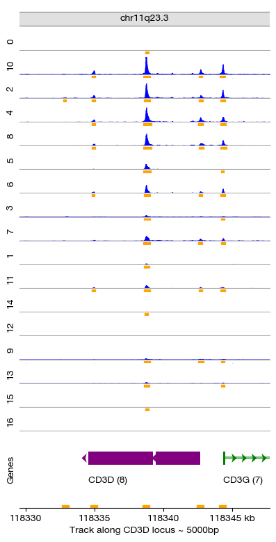
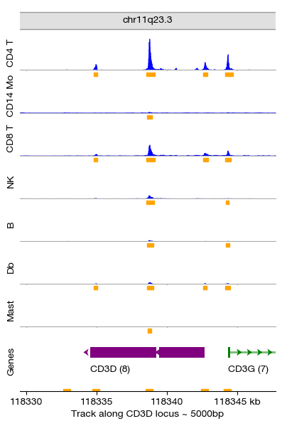
We can observe that the chromatin accessibility landscape varies significantly across cell types, particularly at marker gene loci. Here we visualize the CD3D locus — a canonical T-cell marker gene. The coverage tracks for each Leiden cluster show:
T cell clusters (e.g., clusters 4, 6, 7, 8): High accessibility at the CD3D promoter
Non-T cell clusters (e.g., B cells, monocytes): Minimal accessibility at CD3D
This confirms that the unsupervised clustering has successfully separated cell types based on their chromatin accessibility patterns.
[64]:
import warnings
warnings.filterwarnings('ignore')
[65]:
figs = expm.atac.plot_peaks(
    group_key = 'leiden', peaks_key = 'peaks.leiden',
    # either specifying a gene name for convenience
    gene = 'CD3D', upstream = 5000, downstream = 5000,
    # or specify chromosome coordinates manually
    chr = None, xf = None, xt = None,
    figsize = (4, 8), dpi = 100,
    gene_track_height = 0.15, chrom_track_height = 0.05,
    peak_annotation_height = 0.15,
    min_frag_length = None, max_frag_length = 180,
    title = 'Track along CD3D locus ~ 5000bp', showgn = True,
    plot_consensus_peak = 'peaks.merged',
    do_tight_layout = False,
)
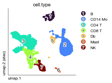
Initial Cell Type Annotation#
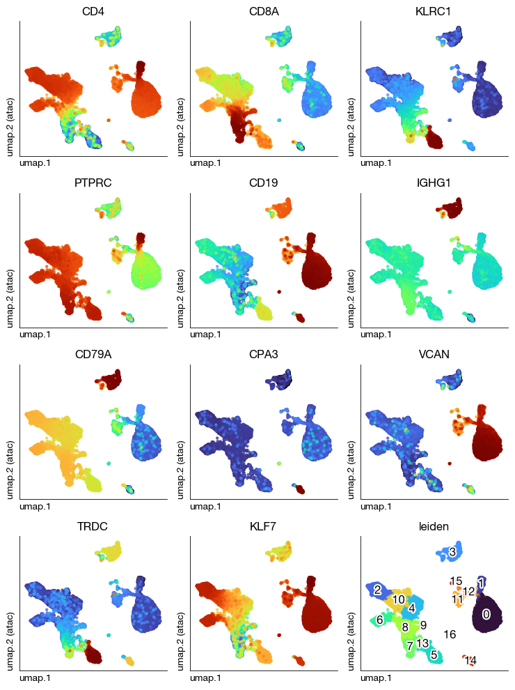
We can annotate cell types based on the inferred gene activity matrix. Marker gene accessibility patterns from ATAC-seq may differ somewhat from RNA expression patterns, but the overall cluster identities are generally concordant. ATAC-seq and RNA-seq provide complementary perspectives on cell identity:
RNA-seq: Measures the transcriptome — what genes are being actively transcribed
ATAC-seq: Measures the epigenome — what regulatory regions are open and poised for transcription
Together, they distinguish between active transcription and poised/primed regulatory states
Annotation strategy:
Visualize known marker genes on the UMAP embedding (using the MAGIC-smoothed matrix)
Identify differentially accessible genes per cluster using DESeq2
Map Leiden clusters to cell types based on marker knowledge
Marker genes used: | Gene | Cell Type | |——|———–| | CD4 | CD4+ T cells | | CD8A | CD8+ T cells | | KLRC1 | NK cells | | PTPRC (CD45) | All immune cells | | CD19, CD79A | B cells | | CD14 | Monocytes | | CPA3 | Mast cells |
[69]:
expm.rna.log_normalize(
    key_source = 'magic',
    run_on_samples = ['atac'],
)
[78]:
fig = expm.rna.plot_multiple_embedding(
    run_on_samples = ['atac'],
    slot = 'X',
    basis = 'umap', figsize = (7.5, 10),
    features = [
        'CD4', 'CD8A', 'KLRC1',
        'PTPRC', 'CD19', 'IGHG1',
        'CD79A', 'CPA3', 'VCAN',
        'TRDC', 'KLF7', 'leiden'
    ], ncols = 3, legend = False, annotate_style = 'text'
)
[ ]:
expm.rna.markers_deseq(
    run_on_samples = ['atac'],
    counts = 'counts',
    metadata = ['sample', 'leiden'], formula = '~ leiden',
    variable = 'leiden', experiment = '6', control = '8',
    key_added = 'markers'
)
[76]:
expm.rna.get_markers(
    run_on_samples = ['atac'],
    slot = 'markers',
)['atac'][['gene', 'mean', 'lfc', 'q', 'names']]
[i] fetched diff `6` over `8` (260 genes)
[76]:
| gene | mean | lfc | q | names | |
|---|---|---|---|---|---|
| 52327 | ACTN1 | 2.481912 | 1.768708 | 8.075114e-140 | rna:hsa:g17763 |
| 11465 | KLF7 | 3.268279 | 1.819304 | 3.773807e-135 | rna:hsa:g35282 |
| 56142 | ARRDC4 | 1.430376 | 2.682143 | 7.747638e-130 | rna:hsa:g21046 |
| 56139 | ENSG00000259199 | 2.193997 | 2.589431 | 1.761828e-128 | rna:hsa:g21043 |
| 29843 | GNAI1 | 0.796094 | 2.993757 | 6.883961e-103 | rna:hsa:g54429 |
| ... | ... | ... | ... | ... | ... |
| 20307 | FBXL7 | 0.193910 | 1.098072 | 1.000000e+00 | rna:hsa:g46677 |
| 31674 | ENSG00000300110 | 0.084500 | 1.331007 | 1.000000e+00 | rna:hsa:g55929 |
| 12338 | ENSG00000229996 | 0.083055 | 1.024768 | 1.000000e+00 | rna:hsa:g36046 |
| 45663 | SLC25A39P2 | 0.054773 | 1.012316 | 1.000000e+00 | rna:hsa:g72986 |
| 29835 | MAGI2-AS3 | 0.053906 | 1.031998 | 1.000000e+00 | rna:hsa:g54423 |
260 rows × 5 columns
[90]:
expm.rna.annotate(
    run_on_samples = ['atac'],
    mapping = {
        'CD14 Mo': [0, 1, 12, 15],
        'Db': [11, 16],
        'B': [3],
        'CD4 T': [2, 4, 10, 6],
        'CD8 T': [8, 7, 13, 9],
        'NK': [5],
        'Mast': [14]
    }
)
cell.type
CD4 T      4006
CD14 Mo    2646
CD8 T      1508
NK          689
B           539
Db          318
Mast        162
Name: count, dtype: int64
[91]:
fig = expm.rna.plot_embedding(
    run_on_samples = ['atac'],
    slot = 'magic',
    basis = 'umap', color = 'cell.type', figsize = (4, 3)
)
[92]:
expm['atac'].obs['cell.type'] = expm.rna['atac'].obs['cell.type']
[93]:
expm.atac.call_peaks_fragments(
    # call peaks from fragments
    groupby = 'cell.type',
    qvalue = 0.05,
    call_broad_peaks = False,
    broad_cutoff = 0.1,
    replicate = None,
    replicate_qvalue = None,
    max_frag_size = 180,  # only call nucleosome-free fragments
    selections = None,
    nolambda = False,
    shift = -100,
    extsize = 200,
    min_len = None,
    blacklist = None,
    # directly call groups of peaks
    key_added = 'peaks.ctype',
    inplace = True,
    n_jobs = 30
)
[i] exporting fragments ...
[i] calling peaks ...
[96]:
figs = expm.atac.plot_peaks(
    group_key = 'cell.type', peaks_key = 'peaks.ctype',
    # either specifying a gene name for convenience
    gene = 'CD3D', upstream = 5000, downstream = 5000,
    # or specify chromosome coordinates manually
    chr = None, xf = None, xt = None,
    figsize = (4, 6), dpi = 100,
    gene_track_height = 0.15, chrom_track_height = 0.075,
    peak_annotation_height = 0.15,
    min_frag_length = None, max_frag_length = 180,
    title = 'Track along CD3D locus ~ 5000bp', showgn = True,
    plot_consensus_peak = 'peaks.merged',
    do_tight_layout = False,
)
Save the Processed Data#
All changes — including QC filters, bin matrices, dimensionality reduction, cluster assignments, gene activity inference, peak calls, and cell type annotations — are saved to disk. The experiment can be reloaded later with em.load_experiment('multiome') without repeating any of the computational steps.
[97]:
print(expm)
annotated data of size 17696 × 75855
annotated data of size 9868 × 6176584
annotated data of size 9868 × 214959
integrated dataset of size 17696 × 6467398
contains modalities: rna, atac, atac-peak

 modality [rna]
    obs : sample <cat> <c/sample> batch <cat> <c/batch> group <cat> <c> modality <cat> <c/modality>
          taxa <cat> <c/taxa> barcode <o> <o> ubc <cat> <o> n.umi <f64> <i> n.genes <f64> <i>
          n.mito <f64> <f> n.ribo <f64> <f> pct.mito <f64> <f> pct.ribo <f64> <f>
          filter <boolean> <bool> score.doublet <f64> <f> score.doublet.se <f64> <f>
          is.doublet <bool> <bool> qc <boolean> <bool/qc> n.fragments <f64> <f> pct.dup <f64> <f>
          tsse <f64> <f> leiden <cat> <o>
    var : chr <cat> <c/chromosome> start <i64> <i> end <i64> <i> strand <cat> <c/strand> id <o> <o>
          subtype <cat> <c/gsubtype> gene <cat> <o/gene> tlen <f64> <i/tlen> cdslen <i64> <i/cdslen>
          assembly <cat> <c> uid <o> <o/ugene>
    uns : slots <system>

 modality [atac]
    obs : n.fragments <ui64> <i> pct.dup <f64> <f> pct.mito <f64> <f> barcode <o> <o> ubc <o> <o>
          sample <cat> <c/sample> batch <cat> <c/batch> group <cat> <c> modality <cat> <c/modality>
          taxa <cat> <c/taxa> tsse <f64> <f/tsse> n.umi <ui64> <i> score.doublet <f64> <f>
          score.doublet.se <f64> <f> is.doublet <bool> <bool> leiden <cat> <c> cell.type <cat>
    var : chr <cat> <c/chromosome> start <cat> <i> end <cat> <i> location <o> <o/location>
          unique <o> <o>
   obsm : paired <csr:ui32(3088286401)> <fragments>
    uns : assembly <assembly> assembly.size <asm-size> slots <system>
          peaks.leiden <dict/peaks/grouped-peaks> commands <system>
          peaks.merged <dict/peaks/merged-peaks> peaks.ctype <dict/peaks/grouped-peaks>

 modality [atac-peak]
    obs : n.fragments <ui64> <i> pct.dup <f64> <f> pct.mito <f64> <f> barcode <o> <o> ubc <o> <o>
          sample <cat> <c/sample> batch <cat> <c/batch> group <cat> <c> modality <cat> <c/modality>
          taxa <cat> <c/taxa> tsse <f64> <f/tsse> n.umi <ui64> <i> score.doublet <f64> <f>
          score.doublet.se <f64> <f> is.doublet <bool> <bool> leiden <cat> <c>
    var : 12 <bool> <bool> 15 <bool> <bool> 6 <bool> <bool> 11 <bool> <bool> 8 <bool> <bool>
          9 <bool> <bool> 2 <bool> <bool> 7 <bool> <bool> 5 <bool> <bool> 3 <bool> <bool>
          16 <bool> <bool> 14 <bool> <bool> 0 <bool> <bool> 13 <bool> <bool> 1 <bool> <bool>
          10 <bool> <bool> 4 <bool> <bool> chr <o> <c/chromosome> start <i64> <i> end <i64> <i>
          strand <o> <o/strand> summit <i64> <i>
    uns : assembly <assembly> assembly.size <asm-size> slots <system> commands <system>

[*] composed of samples:
  atac    atac  hsa/grch38   batch b-1     of size 9868 × 6176584
  gex     rna   hsa/grch38   batch b-1     of size 7828 × 24898
  atac    rna   hsa/grch38   batch b-1     of size 9868 × 75716
[99]:
expm.save()
[i] main dataset write to expm/multiome/integrated.h5mu
[i] saving individual samples. (pass `save_samples = False` to skip)
   ━━━━━━━━━━━━━━━━━━━━━━━━━━ modality [atac]          1 / 1     (00:36 < 00:00)
   ━━━━━━━━━━━━━━━━━━━━━━━━━━ modality [rna]           2 / 2     (01:37 < 00:00)
   ━━━━━━━━━━━━━━━━━━━━━━━━━━ modality [atac-peak]     1 / 1     (00:01 < 00:00)