Spatial Domain Identification#

Spatial transcriptomics data from bin-based platforms like Visium captures gene expression across tissue sections without single-cell resolution, where each spot may contain multiple cells. Identifying spatial domains — contiguous tissue regions with distinct molecular signatures — is a key analytical goal that reveals tissue architecture and microenvironment organization. This notebook demonstrates spatial domain identification using the exprmat package with multiple complementary algorithms. We cover spatially variable gene detection with SpatialDE, domain detection using SpaGCN with and without histological image integration, and deep learning-based domain identification with DeepST. We also demonstrate integration of spatial domains across multiple samples and the identification of domain-specific marker genes.

[1]:

%load_ext autoreload
%autoreload 2

[2]:

import exprmat as em
em.setwd('../../../data')
ver = em.version()

[i] exprmat 0.2.66 / exprmat-db 0.2.66
[i] os: posix (linux)  platform version: 6.8.0-90-generic
[i] loaded configuration from /home/data/yangz/.exprmatrc
[i] current working directory: /home/data/yangz/packages/exprmat/data
[i] current database directory: /home/data/yangz/packages/database (0.2.66)
[i] resident memory: 777.58 MiB
[i] virtual memory: 5.95 GiB

[3]:

expm = em.load_experiment('expm/visium')

   ━━━━━━━━━━━━━━━━━━━━━━━━━━ loading samples          8 / 8     (00:06 < 00:00)

Identification of spatial domains is commonly useful in bin-based data. Since this gives an abstraction of cellular neighborhood in spatial coordinates. For single cell resolution expression matrices, a direct approach of cellular neighbors binning after cell type identification is more accurate and meaningful, (see tutorial d1 and e1) though the same algorithm still works, it is not a recommended workflow.

[6]:

print(expm)

annotated data of size 12038 × 35554
integrated dataset of size 12038 × 35554
contains modalities: spatial-bin

 modality [spatial-bin]
    obs : sample <cat> batch <cat> group <cat> modality <cat> taxa <cat> barcode <o> ubc <o>
          in.tissue <i64> row <i64> col <i64> y <i64> x <i64>
    var : chr <cat> start <i64> end <i64> strand <cat> id <o> subtype <cat> gene <cat> tlen <f64>
          cdslen <i64> assembly <cat> uid <o>
   obsm : spatial <arr:i64(2)>
    uns : spatial

[*] composed of samples:
  p1-t4    spatial-bin hsa    batch b1      of size 1155 × 35554
  p1-t5    spatial-bin hsa    batch b2      of size 1726 × 35554
  p1-t7    spatial-bin hsa    batch b3      of size 1191 × 35554
  p1-t10   spatial-bin hsa    batch b4      of size 1522 × 35554
  p2-t1    spatial-bin hsa    batch b5      of size 2197 × 35554
  p2-t2    spatial-bin hsa    batch b6      of size 1853 × 35554
  p2-t5    spatial-bin hsa    batch b7      of size 1470 × 35554
  p2-t6    spatial-bin hsa    batch b8      of size 924 × 35554

SpatialDE#

Identification of spatially variable genes is often performed sample-wise. Before merged to the whole dataset. SpatialDE requires counts layer input

[5]:

sample = 'p2-t5'

[8]:

expm.spatial_bin.view(sample)

annotated data of size 1470 × 35554
    obs : sample <cat> batch <cat> group <cat> modality <cat> taxa <cat> barcode <o> ubc <o>
          in.tissue <i64> row <i64> col <i64> y <i64> x <i64> leiden <cat>
    var : chr <cat> start <i64> end <i64> strand <cat> id <o> subtype <cat> gene <cat> tlen <f64>
          cdslen <i64> assembly <cat> uid <o> vst.means <f64> vst.vars <f64> vst.vars.norm <f64>
          vst.hvg.rank <f32> vst.hvg <bool>
 layers : counts <f32> lognorm <f32> norm <f32>
   obsm : knn <arr:i32(30)> knn.d <arr:f64(30)> pca <arr:f64(35)> spatial <arr:i64(2)>
          spatial.array <arr:i64(2)> umap <arr:f32(2)>
   varm : pca <arr:f64(35)>
   obsp : connectivities <csr:f32> distances <csr:f64>
    uns : leiden neighbors pca spatial umap

[9]:

expm.spatial_bin.spatial_svg_spatialde(
    run_on_samples = [sample],
    layer = 'counts',
    spatial_key = 'spatial',
    kernel_space = None,
    sizefactors = None,
    obs_dist = 'negative_binomial',
    use_cache = True,
    use_gpu = True,
    progress = True,
    n_svg = 500,
    key_added = 'spatialde'
)

[i] performing spatialde score test for svgs ...

   ━━━━━━━━━━━━━━━━━━━━━━━━━━ spatialde score test 35554 / 35554 (05:13 < 00:00)

[i] tested 35554 genes; 1845 significant at fdr 5%.

[9]:

{'p2-t5': None}

[15]:

expm.spatial_bin[sample].var[['gene', 'spatialde.padj', 'spatialde.svg', 'spatialde.rank']] \
    .sort_values('spatialde.rank').head(15)

[15]:

	gene	spatialde.padj	spatialde.svg	spatialde.rank
rna:hsa:g38601	CSTB	5.124839e-11	True	1.0
rna:hsa:g11501	HSPA8	5.124839e-11	True	2.0
rna:hsa:g52277	PERP	5.124839e-11	True	3.0
rna:hsa:g57815	PABPC1	5.124839e-11	True	4.0
rna:hsa:g57829	YWHAZ	5.124839e-11	True	5.0
rna:hsa:g31642	CMPK2	5.124839e-11	True	6.0
rna:hsa:g31643	RSAD2	5.124839e-11	True	7.0
rna:hsa:g16460	COL4A1	5.124839e-11	True	8.0
rna:hsa:g19674	DUOX2	5.124839e-11	True	9.0
rna:hsa:g19675	DUOXA2	5.124839e-11	True	10.0
rna:hsa:g19696	C15orf48	5.124839e-11	True	11.0
rna:hsa:g19654	B2M	5.124839e-11	True	12.0
rna:hsa:g45142	RPL34	5.124839e-11	True	13.0
rna:hsa:g44891	SPP1	5.124839e-11	True	14.0
rna:hsa:g38502	MX2	5.124839e-11	True	15.0

[28]:

fig = expm.spatial_bin.plot_spatial(
    run_on_samples = [sample],
    channels = ['hires/r', 'hires/g', 'hires/b'],
    plot_embeddings = {
        'visible': True,
        'basis': 'spatial',
        'color': 'CSTB',
        'ptsize': 15,
    },
    xrange = (3000, 13000),
    yrange = (5000, 15000),
    figsize = (5, 5)
)

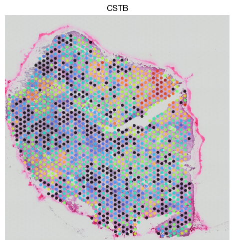
../_images/spatial_f1-spatial-domains_13_0.png

Such spatially variable gene can be intersected to highly variable genes to perform HVG selection and later dimensionality reduction process with spatially-awared properties

Spatial domain identification#

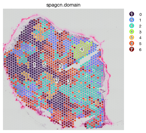
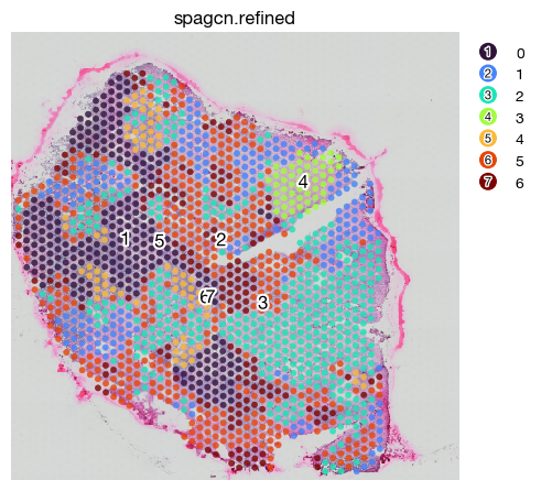
Several methods are available to identify spatial domains with similar expression profile beforehand, and then infer gene signature of those domains. These offer visually explainable gene signatures with direct mapping to tissue distribution.

SpaGCN provides a robust implementation of such algorithms. It requires a normalized expression matrix to fit the model. User should have a estimated number of clusters and may run the method several time to achieve requested resolution. An H&E image may also be provided for image embeddings

[37]:

expm.spatial_bin.spatial_detect_domains_spagcn(
    run_on_samples = [sample],
    layer = 'lognorm',
    channels = None,
    n_clusters = 7,
    histology = False,  # at present without histology images.
    refine_shape = 'hexagon',
    seed = 42,
    key_added = 'spagcn.domain',
    refined_key_added = 'spagcn.refined'
)

[i] calculating adjacency matrix from xy coordinates only.
[i] recommended l = 90.829404296875
[i] search_res starting at res = 0.70, step = 0.10.
[i] res = 0.60, n_clusters = 8.
[i] delta_label 0.004762 < tol 0.005, stopping at epoch 19.
[i] res = 0.50, n_clusters = 5.
[i] res = 0.55, n_clusters = 8.
[i] delta_label 0.004762 < tol 0.005, stopping at epoch 19.
[i] res = 0.50, n_clusters = 5.
[i] res = 0.52, n_clusters = 8.
[i] delta_label 0.004762 < tol 0.005, stopping at epoch 19.
[i] res = 0.50, n_clusters = 5.
[i] res = 0.51, n_clusters = 8.
[i] delta_label 0.004762 < tol 0.005, stopping at epoch 19.
[i] res = 0.50, n_clusters = 5.
[i] res = 0.51, n_clusters = 7.
[i] delta_label 0.004762 < tol 0.005, stopping at epoch 22.
[i] calculating adjacency matrix from xy coordinates only.

[31]:

fig = expm.spatial_bin.plot_spatial(
    run_on_samples = [sample],
    channels = ['hires/r', 'hires/g', 'hires/b'],
    plot_embeddings = {
        'visible': True,
        'basis': 'spatial',
        'color': 'spagcn.domain',
        'ptsize': 15,
    },
    xrange = (3000, 13000),
    yrange = (5000, 15000),
    figsize = (5, 5)
)

../_images/spatial_f1-spatial-domains_18_0.png

[32]:

fig = expm.spatial_bin.plot_spatial(
    run_on_samples = [sample],
    channels = ['hires/r', 'hires/g', 'hires/b'],
    plot_embeddings = {
        'visible': True,
        'basis': 'spatial',
        'color': 'spagcn.refined',
        'ptsize': 15,
    },
    xrange = (3000, 13000),
    yrange = (5000, 15000),
    figsize = (5, 5)
)

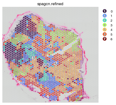
../_images/spatial_f1-spatial-domains_19_0.png

You may also retrieve the high-resolution tissue image to faciliate tissue-morphology based spatial domain identification

[39]:

he = expm.spatial_bin.get_image(
    run_on_samples = ['p1-t4'],
    channels = ['hires/r', 'hires/g', 'hires/b']
)

[36]:

expm.spatial_bin.spatial_detect_domains_spagcn(
    run_on_samples = [sample],
    layer = 'lognorm',
    channels = ['hires/r', 'hires/g', 'hires/b'],
    n_clusters = 7,
    histology = True,
    refine_shape = 'hexagon',
    seed = 42,
    key_added = 'spagcn.domain',
    refined_key_added = 'spagcn.refined'
)

[i] calculating adjacency matrix from spatial coords + histology image.
[i] recommended l = 121.1025390625
[i] search_res starting at res = 0.70, step = 0.10.
[i] res = 0.60, n_clusters = 8.
[i] res = 0.50, n_clusters = 6.
[i] res = 0.55, n_clusters = 7.
[i] delta_label 0.004082 < tol 0.005, stopping at epoch 43.
[i] calculating adjacency matrix from xy coordinates only.

[34]:

fig = expm.spatial_bin.plot_spatial(
    run_on_samples = [sample],
    channels = ['hires/r', 'hires/g', 'hires/b'],
    plot_embeddings = {
        'visible': True,
        'basis': 'spatial',
        'color': 'spagcn.refined',
        'ptsize': 15,
    },
    xrange = (3000, 13000),
    yrange = (5000, 15000),
    figsize = (5, 5)
)

../_images/spatial_f1-spatial-domains_23_0.png

Spatial domain identification using DeepST#

DeepST provides an alternative to SpaGCN. Though the result is less convincing in this case.

[38]:

expm.spatial_bin.spatial_detect_domains_deepst(
    run_on_samples = [sample],
    image_key = 'hires',
    n_domains = 7,
    use_image = False,
    save_path = './expm/deepst',
    pre_epochs = 200,
    epochs = 200,
    use_gpu = True
)

[i] spatial weights computed; average neighbours = 30.0.
[i] gene-expression weights computed.
[i] combined weight matrix saved to adata.obsm['weights'].

   ━━━━━━━━━━━━━━━━━━━━━━━━ finding adjacent spots  1470 / 1470  (00:01 < 00:00)

[i] data augmentation completed.
[i] 12.0000 neighbours per cell on average.
[i] spatial graph computation completed.
[i] running deepst training ...

   ━━━━━━━━━━━━━━━━━━━━━ pretraining initial model   200 / 200   (00:05 < 00:00)
   ━━━━━━━━━━━━━━━━━━━━━━━━━━ training final model   200 / 200   (00:05 < 00:00)

[i] deepst training finished. memory usage = 4.58 GB; total time = 0.20 min.
[i] found resolution 0.41 for 7 domains.
[i] deepst domain detection complete.

[39]:

expm.spatial_bin.view(sample)

annotated data of size 1470 × 35554
    obs : sample <cat> batch <cat> group <cat> modality <cat> taxa <cat> barcode <o> ubc <o>
          in.tissue <i64> row <i64> col <i64> y <i64> x <i64> leiden <cat> spagcn.domain <cat>
          spagcn.refined <cat> imagerow <f64> imagecol <f64> deepst.domain <cat>
          deepst.refined <cat>
    var : chr <cat> start <i64> end <i64> strand <cat> id <o> subtype <cat> gene <cat> tlen <f64>
          cdslen <i64> assembly <cat> uid <o> vst.means <f64> vst.vars <f64> vst.vars.norm <f64>
          vst.hvg.rank <f32> vst.hvg <bool> spatialde.padj <f64> spatialde.svg <bool>
          spatialde.rank <f64>
 layers : counts <f32> lognorm <f32> norm <f32>
   obsm : knn <arr:i32(30)> knn.d <arr:f64(30)> pca <arr:f64(35)> spatial <arr:i64(2)>
          spatial.array <arr:i64(2)> umap <arr:f32(2)> weights <arr:f64> adjacent <arr:f64(35554)>
          augmented.genes <arr:f64(35554)> deepst.embedding <arr:f32(28)>
   varm : pca <arr:f64(35)>
   obsp : connectivities <csr:f32> distances <csr:f64>
    uns : leiden neighbors pca spatial umap deepst.domain

[40]:

fig = expm.spatial_bin.plot_spatial(
    run_on_samples = [sample],
    channels = ['hires/r', 'hires/g', 'hires/b'],
    plot_embeddings = {
        'visible': True,
        'basis': 'spatial',
        'color': 'deepst.refined',
        'ptsize': 15,
    },
    xrange = (3000, 13000),
    yrange = (5000, 15000),
    figsize = (5, 5)
)

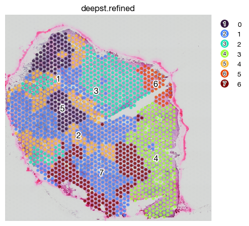
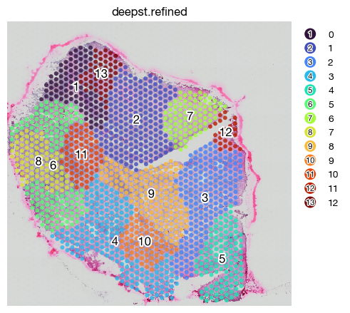
../_images/spatial_f1-spatial-domains_27_0.png

I do not recommend running DeepST on data other than large bins, since the intermediate storage of per-spot image clips may occupy much storage for cells greater than 5000.

[41]:

expm.spatial_bin.spatial_detect_domains_deepst(
    run_on_samples = [sample],
    image_key = 'hires',
    n_domains = 7,
    use_image = True,
    save_path = './expm/deepst',
    pre_epochs = 3000,
    epochs = 3000,
    use_gpu = True
)

   ━━━━━━━━━━━━━━━━━━━━━━━━━━ cropping spot images  1470 / 1470  (00:38 < 00:00)
   ━━━━━━━━━━━━━━━━━━━━━ extracting image features  1470 / 1470  (00:17 < 00:00)

[i] spatial weights computed; average neighbours = 30.0.
[i] gene-expression weights computed.
[i] morphological weights computed.
[i] combined weight matrix saved to adata.obsm['weights'].

   ━━━━━━━━━━━━━━━━━━━━━━━━ finding adjacent spots  1470 / 1470  (00:01 < 00:00)

[i] data augmentation completed.
[i] 12.0000 neighbours per cell on average.
[i] spatial graph computation completed.
[i] running deepst training ...

   ━━━━━━━━━━━━━━━━━━━━━ pretraining initial model  3000 / 3000  (01:15 < 00:00)
   ━━━━━━━━━━━━━━━━━━━━━━━━━━ training final model  3000 / 3000  (01:29 < 00:00)

[i] deepst training finished. memory usage = 5.21 GB; total time = 2.75 min.
[!] no resolution gave exactly 7 domains; falling back to resolution = 0.2.
[i] deepst domain detection complete.

[42]:

fig = expm.spatial_bin.plot_spatial(
    run_on_samples = [sample],
    channels = ['hires/r', 'hires/g', 'hires/b'],
    plot_embeddings = {
        'visible': True,
        'basis': 'spatial',
        'color': 'deepst.refined',
        'ptsize': 15,
    },
    xrange = (3000, 13000),
    yrange = (5000, 15000),
    figsize = (5, 5)
)

../_images/spatial_f1-spatial-domains_30_0.png

Integrating multiple datasets to uniformed domains#

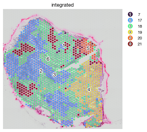
Spatial integration are often useful to identify patterns shared across different samples. This generalizability provides an easy access to comparisons. Since DeepST did not perform well on tumor tissues, we prefer SpaGCN integration of domains.

[ ]:

expm.spatial_bin.integrate_domains_spagcn(
    n_clusters = 15,
    run_on_samples = True, # integrate all samples.
    result_key = 'integrated',
    histology = False,
    max_epochs = 500,
    seed = 100,
)

[i] delta_label 0.004901 < tol 0.005, stopping at epoch 70.

[45]:

fig = expm.spatial_bin.plot_spatial(
    run_on_samples = [sample],
    channels = ['hires/r', 'hires/g', 'hires/b'],
    plot_embeddings = {
        'visible': True,
        'basis': 'spatial',
        'color': 'integrated',
        'ptsize': 15,
    },
    xrange = (3000, 13000),
    yrange = (5000, 15000),
    figsize = (5, 5)
)

../_images/spatial_f1-spatial-domains_34_0.png

Identify domain-specific markers#

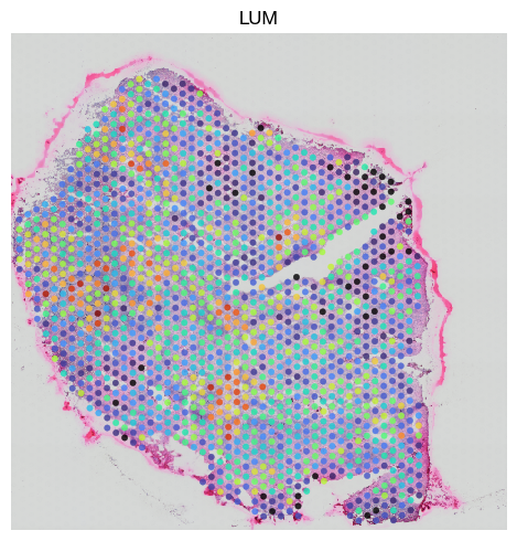
Like we obtain marker from unsupervised clustering, such spatial domains can use specially designed methods for marker gene retrieval

[ ]:

expm.spatial_bin.spatial_markers_spagcn(
    run_on_samples = [sample],
    domain_key = 'integrated',
    min_in_group_fraction = 0.8,
    min_in_out_group_ratio = 1,
    min_fold_change = 1.5,
    num_neighbours = 3,
    ratio = 0.5,
    radius_quantiles = (0.001, 0.1),
    num_min = 10,
    num_max = 14,
    max_run = 100,
    key_added = 'spagcn.markers'
)

[ ]:

expm.spatial_bin.get_markers(
    run_on_samples = [sample],
    slot = 'spagcn.markers',
    group_name = '17'
)[sample][['gene', 'pct.in', 'pct.out', 'fc', 'q', 'log10.q']]

[i] fetched diff `17` over `rest` (18 genes)

	gene	pct.in	pct.out	fc	q	log10.q
rna:hsa:g13826	LUM	1.000000	0.996835	2.302415	6.437318e-78	77.191295
rna:hsa:g22861	HERPUD1	0.997691	0.995253	2.107135	6.339839e-77	76.197922
rna:hsa:g53680	SFRP4	0.852194	0.485759	2.073682	2.236636e-110	109.650405
rna:hsa:g15444	POSTN	0.946882	0.783228	1.945651	3.066666e-95	94.513333
rna:hsa:g57703	TP53INP1	0.997691	0.992089	1.802479	7.859763e-72	71.104591
rna:hsa:g59915	ASPN	0.967667	0.799051	1.755815	1.035827e-91	90.984713
rna:hsa:g57902	CTHRC1	0.963048	0.806962	1.665744	3.148795e-84	83.501856
rna:hsa:g6228	VIM	1.000000	0.995253	1.655484	1.246817e-58	57.904197
rna:hsa:g4692	BTG2	0.997691	0.995253	1.605542	1.204427e-58	57.919219
rna:hsa:g62036	PIM2	0.995381	0.985759	1.579871	1.728512e-58	57.762328
rna:hsa:g45757	SFRP2	0.933025	0.912975	1.579464	7.928045e-74	73.100834
rna:hsa:g35422	IGFBP5	0.956120	0.943038	1.578879	2.130125e-68	67.671595
rna:hsa:g58420	PTP4A3	1.000000	0.985759	1.565828	1.001160e-74	73.999496
rna:hsa:g39969	FBLN1	0.935335	0.881329	1.562546	6.522984e-76	75.185554
rna:hsa:g52137	CCN2	0.995381	0.988924	1.557651	3.224739e-44	43.491505
rna:hsa:g35923	COL6A3	0.990762	0.973101	1.552273	5.541407e-72	71.256380
rna:hsa:g44744	CXCL13	0.956120	0.941456	1.518375	1.463188e-57	56.834700
rna:hsa:g34966	COL5A2	0.997691	0.977848	1.515412	1.668277e-65	64.777732

[57]:

fig = expm.spatial_bin.plot_spatial(
    run_on_samples = [sample],
    channels = ['hires/r', 'hires/g', 'hires/b'],
    plot_embeddings = {
        'visible': True,
        'basis': 'spatial',
        'color': 'LUM',
        'ptsize': 15,
    },
    xrange = (3000, 13000),
    yrange = (5000, 15000),
    figsize = (5, 5)
)

../_images/spatial_f1-spatial-domains_38_0.png

Detect metagenes#

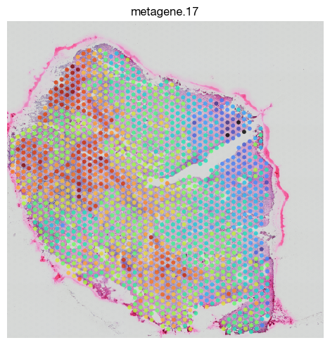
SpaGCN provides a simple linear model of gene combinations to introduce high specificity marker set as metagenes

[11]:

expm.spatial_bin.spatial_metagene(
    run_on_samples = [sample],
    domain_key = 'integrated',
    target_cluster = '17',
    key_svg = 'spagcn.markers',
    max_iter = 6,
    key_added = 'metagene.17'
)

[i] add gene: rna:hsa:g18771; minus gene: rna:hsa:g3509
[i] absolute mean change: 4.9681
[i] non-target spots reduced to: 149
[i] meta gene now: rna:hsa:g58420 + rna:hsa:g18771 - rna:hsa:g3509
[i] add gene: rna:hsa:g39127; minus gene: rna:hsa:g53115
[i] absolute mean change: 7.4248
[i] non-target spots reduced to: 10
[i] meta gene now: rna:hsa:g58420 + rna:hsa:g18771 - rna:hsa:g3509 + rna:hsa:g39127 - rna:hsa:g53115
[i] meta gene: rna:hsa:g58420 + rna:hsa:g18771 - rna:hsa:g3509 + rna:hsa:g39127 - rna:hsa:g53115
[i] meta gene: rna:hsa:g58420 + rna:hsa:g18771 - rna:hsa:g3509 + rna:hsa:g39127 - rna:hsa:g53115

[13]:

fig = expm.spatial_bin.plot_spatial(
    run_on_samples = [sample],
    channels = ['hires/r', 'hires/g', 'hires/b'],
    plot_embeddings = {
        'visible': True,
        'basis': 'spatial',
        'color': 'metagene.17',
        'ptsize': 15,
    },
    xrange = (3000, 13000),
    yrange = (5000, 15000),
    figsize = (5, 5)
)

../_images/spatial_f1-spatial-domains_41_0.png

[17]:

expm.spatial_bin.view(sample)

annotated data of size 1470 × 35554
    obs : sample <cat> batch <cat> group <cat> modality <cat> taxa <cat> barcode <o> ubc <o>
          in.tissue <i64> row <i64> col <i64> y <i64> x <i64> leiden <cat> spagcn.domain <cat>
          spagcn.refined <cat> imagerow <f64> imagecol <f64> deepst.domain <cat>
          deepst.refined <cat> integrated <cat> metagene.17 <f64>
    var : chr <cat> start <i64> end <i64> strand <cat> id <o> subtype <cat> gene <cat> tlen <f64>
          cdslen <i64> assembly <cat> uid <o> vst.means <f64> vst.vars <f64> vst.vars.norm <f64>
          vst.hvg.rank <f32> vst.hvg <bool> spatialde.padj <f64> spatialde.svg <bool>
          spatialde.rank <f64>
 layers : counts <f32> lognorm <f32> norm <f32>
   obsm : adjacent <arr:f64(35554)> augmented.genes <arr:f64(35554)> deepst.embedding <arr:f32(28)>
          knn <arr:i32(30)> knn.d <arr:f64(30)> pca <arr:f64(35)> spatial <arr:i64(2)>
          spatial.array <arr:i64(2)> umap <arr:f32(2)> weights <arr:f64>
   varm : pca <arr:f64(35)>
   obsp : connectivities <csr:f32> distances <csr:f64>
    uns : deepst.domain leiden neighbors pca spagcn.markers spatial umap

[18]:

expm.save()

[i] main dataset write to expm/visium/integrated.h5mu
[i] saving individual samples. (pass `save_samples = False` to skip)

   ━━━━━━━━━━━━━━━━━━━━━━━━ modality [spatial-bin]     8 / 8     (00:07 < 00:00)