Clustering and Annotation#
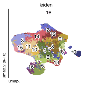
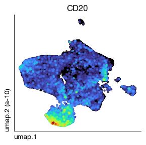
After quantifying marker expression from segmented multiplex immunofluorescence data, the next step is to identify distinct cell populations through clustering and assign biological annotations to each cluster. This notebook demonstrates the clustering and annotation workflow using the exprmat package for CODEX data. We perform PCA-based dimensionality reduction on the compensated marker intensities, construct nearest-neighbor graphs, apply Leiden clustering, and visualize results in both UMAP space and the original tissue coordinates. Manual annotation based on marker expression profiles is followed by label transfer using a trained SVM classifier to propagate annotations across additional samples without manual effort.
[1]:
%load_ext autoreload
%autoreload 2
[2]:
import exprmat as em
em.setwd('../../../data')
ver = em.version()
[i] exprmat 0.2.66 / exprmat-db 0.2.66
[i] os: posix (linux)  platform version: 6.8.0-90-generic
[i] loaded configuration from /home/data/yangz/.exprmatrc
[i] current working directory: /home/data/yangz/packages/exprmat/data
[i] current database directory: /home/data/yangz/packages/database (0.2.66)
[i] resident memory: 777.61 MiB
[i] virtual memory: 5.95 GiB
From my experience, leiden and UMAP won’t work perfectly when merging all the slides together before clustering and annotation. Maybe due to the heterogeneic nature overwhelms the cluster differences even after integration. I personally recommend annotate per slide. If this work is too heavy, a machine learning transfer can be utilized with considerable accuracy, or just tell an agent to do the repetitive work.
Per-slide clustering#
Load the previously quantified CODEX experiment. The compensated marker intensities will be used as the expression basis for clustering.
[3]:
expm = em.load_experiment('expm/codex')
━━━━━━━━━━━━━━━━━━━━━━━━━━ loading samples 2 / 2 (00:00 < 00:00)
[!] integrated mudata object is not generated.
For CODEX data, it is obvious that all channels must be taken into account.
[7]:
expm.spatial_cell.select_hvg(
    run_on_samples = True,
    key_lognorm = 'compensated',
    method = 'vst',
    dest = 'vst',
)
[!] only 59 genes detected
[!] skipping hvg selection and flagging all as highly variable.
[!] only 59 genes detected
[!] skipping hvg selection and flagging all as highly variable.
Select highly variable markers from the compensated intensity matrix. For CODEX data, all protein channels are biologically relevant, so the HVG selection identifies markers with the most dynamic range across cells rather than filtering out uninformative features.
[8]:
expm.spatial_cell.scale_pca(
    run_on_samples = True,
    hvg = 'vst.hvg',
    key_lognorm = 'compensated',
    key_scaled = 'scaled',
    key_added = 'pca', n_comps = 12,
    keep_sparse = True,
    random_state = 42,
    svd_solver = 'arpack'
)
Scale the marker intensities and compute PCA. With only ~30-60 protein markers in a typical CODEX panel, we use a small number of principal components (12) to capture the major axes of protein expression variation while avoiding overfitting.
[9]:
expm.spatial_cell.knn(
    run_on_samples = True,
    use_rep = 'pca',
    n_comps = None,
    n_neighbors = 30,
    knn = True,
    method = "umap",
    transformer = None,
    metric = "cosine",
    metric_kwds = {},
    random_state = 42,
    key_added = 'neighbors',
    use_gpu = True
)
Construct a KNN graph on the PCA embedding using cosine distance. This graph captures cell-cell similarity in protein expression space, which will be used for graph-based clustering and UMAP visualization.
[27]:
expm.spatial_cell.leiden(
    run_on_samples = True,
    resolution = 1,
    restrict_to = None,
    random_state = 42,
    key_added = 'leiden',
    adjacency = None,
    directed = None,
    use_weights = True,
    n_iterations = 2,
    partition_type = None,
    neighbors_key = None,
    obsp = None,
    flavor = 'igraph',
    use_gpu = True
)
Apply Leiden clustering at resolution 1.0 to identify cell populations. The relatively high resolution ensures that rare but distinct cell types (e.g., NK cells, endothelial cells) are resolved as separate clusters rather than being merged into broader categories.
[11]:
expm.spatial_cell.umap(
    run_on_samples = True,
    min_dist = 0.1,
    spread = 3,
    n_components = 2,
    maxiter = 2000,
    alpha = 1,
    gamma = 1,
    negative_sample_rate = 5,
    init_pos = "random",
    random_state = 42,
    a = None, b = None,
    key_added = 'umap',
    neighbors_key = "neighbors",
    use_gpu = True
)
Compute UMAP embedding for visualizing the protein-based clusters in 2D. The spread parameter (3) produces a more dispersed layout, helping to separate closely related cell populations.
[28]:
fig = expm.spatial_cell.plot_embedding(
    run_on_samples = ['a-10'],
    basis = 'umap', color = 'leiden', cmap = 'category20b',
    sort = True, figsize = (3, 3), dpi = 100, legend = False, annotate_style = 'text'
)
[18]:
fig = expm.spatial_cell.plot_embedding(
    run_on_samples = ['a-10'],
    basis = 'umap', color = 'CD20', cmap = 'turbo',
    sort = True, figsize = (3, 3), dpi = 100, legend = False
)
[42]:
expm.spatial_cell.view('a-10')
annotated data of size 40485 × 59
    obs : segment <i32> x <f64> y <f64> pixellated <o> smoothened <o> area <f64> circularity <f64>
          qc <bool> leiden <cat>
    var : channel <o> qc <bool> vst.hvg <bool> gene <o>
 layers : compensated <f32> means <f32>
   obsm : segment <df> spatial <arr:f64(2)> pca <arr:f32(12)> knn <arr:i32(30)> knn.d <arr:f32(30)>
          umap <arr:f32(2)>
   varm : pca <arr:f64(12)>
   obsp : connectivities <csr:f32> distances <csr:f32>
    uns : spatial pca neighbors leiden umap leiden.colors
[40]:
for x in expm.all_samples('spatial-cell'):
    expm.spatial_cell[x].X = expm.spatial_cell[x].layers['compensated']
Manual annotation and label transfer#
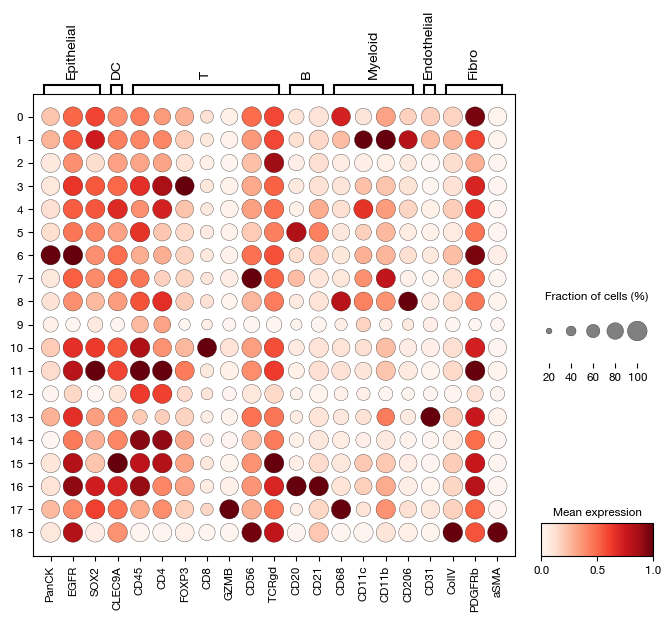
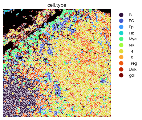
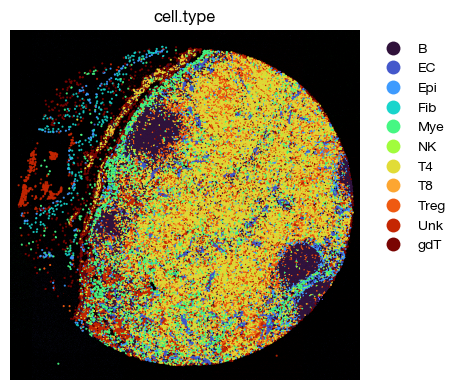
After unsupervised clustering, we assign cell type labels by examining the expression profiles of canonical lineage markers across the Leiden clusters. A dotplot visualization helps identify which markers define each cluster. Based on the expression patterns, we create a mapping from cluster IDs to biological cell types. Once one slide is manually annotated, we train an SVM classifier on the labeled cells and transfer the annotations to the remaining slides, avoiding repetitive manual labeling.
[43]:
fig = expm.spatial_cell.plot_dot(
    run_on_samples = ['a-10'],
    var_names = {
        'Epithelial': ['PanCK', 'EGFR', 'SOX2'],
        'DC': ['CLEC9A'],
        'T': ['CD45', 'CD4', 'FOXP3', 'CD8', 'GZMB', 'CD56', 'TCRgd'],
        'B': ['CD20', 'CD21'],
        'Myeloid': ['CD68', 'CD11c', 'CD11b', 'CD206'],
        'Endothelial': ['CD31'],
        'Fibro': ['ColIV', 'PDGFRb', 'aSMA'],
    },
    groupby = 'leiden', figsize = (8, 6),
    cmap = 'reds/r'
)
[ ]:
expm.spatial_cell.annotate(
    run_on_samples = ['a-10'],
    annotation = 'cell.type',
    mapping = {
        'Fib': [18],
        'B': [16, 5],
        'Mye': [17, 8, 1],
        'NK': [7],
        'Epi': [6],
        'T4': [14, 15, 11, 12, 4],
        'T8': [10],
        'gdT': [2],
        'Treg': [3],
        'EC': [13],
        'Unk': [0, 9],
    },
    cluster = 'leiden'
)
[50]:
fig = expm.spatial_cell.plot_spatial(
    run_on_samples = ['a-10'],
    channels = ['adjusted/cd4', 'adjusted/cd8', 'adjusted/cd20'],
    channel_colors = ['red', 'green', "#5151ffac"],
    plot_embeddings = {
        'visible': True,
        'color': 'cell.type',
        'ptsize': 2,
        'cmap': 'turbo',
        'slot': 'compensated',
        'annotate': False,
        'legend': False
    },
    plot_cells = {
        'visible': True,
        # plot cell boundary
        'key_boundary': 'smoothened',
        'color': 'cell.type',
        'subset': None,
        'alpha': 1,
        'filled': True,
        'palette': 'turbo',
        'legend': True,
    },
    xrange = (1500, 2500),
    yrange = (2500, 3500),
    figsize = (6, 4),
    ticks = False,
    dpi = 100
)
[52]:
fig = expm.spatial_cell.plot_spatial(
    run_on_samples = ['a-10'],
    channels = ['adjusted/cd4', 'adjusted/cd8', 'adjusted/cd20'],
    channel_colors = ['red', 'green', "#5151ffac"],
    plot_embeddings = {
        'visible': True,
        'color': 'cell.type',
        'ptsize': 2,
        'cmap': 'turbo',
        'slot': 'compensated',
        'annotate': False,
        'legend': False
    },
    plot_cells = {
        'visible': True,
        # plot cell boundary
        'key_boundary': 'smoothened',
        'color': 'cell.type',
        'subset': None,
        'alpha': 1,
        'linewidth': 0,
        'filled': True,
        'palette': 'turbo',
        'legend': True,
    },
    figsize = (6, 4),
    ticks = False,
    dpi = 100
)
Label transfer#
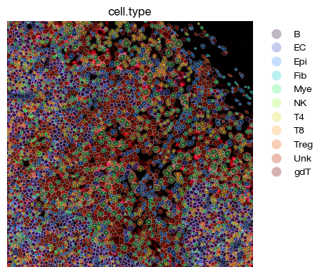
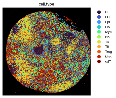
Since we have annotated one sample, let’s transfer to the other to skip manual labeling
[53]:
svm = expm.spatial_cell.train_classifier(
    run_on_samples = ['a-10'],
    label_col = 'cell.type',
    test_size = 0.2,
    random_state = 0,
    mode = 'accurate_svc',
)
[i] unique labels: ['B' 'EC' 'Epi' 'Fib' 'Mye' 'NK' 'T4' 'T8' 'Treg' 'Unk' 'gdT']
[i] training classifier
[i] evaluating classifier
[i] classification accuracy: 0.660
Train a support vector machine (SVM) classifier on the manually annotated cells from slide a-10. The SVM learns a decision boundary in the PCA space that separates the annotated cell types. We reserve 20% of the cells for testing to evaluate classification accuracy before applying the model to unseen slides.
[55]:
svm['a-10']
[55]:
SVC(kernel='linear', probability=True)In a Jupyter environment, please rerun this cell to show the HTML representation or trust the notebook.
On GitHub, the HTML representation is unable to render, please try loading this page with nbviewer.org.
Parameters
| C | 1.0 | |
| kernel | 'linear' | |
| degree | 3 | |
| gamma | 'scale' | |
| coef0 | 0.0 | |
| shrinking | True | |
| probability | True | |
| tol | 0.001 | |
| cache_size | 200 | |
| class_weight | None | |
| verbose | False | |
| max_iter | -1 | |
| decision_function_shape | 'ovr' | |
| break_ties | False | |
| random_state | None |
[56]:
expm.spatial_cell.predict_classifier(
    run_on_samples = ['a-11'],
    clf = svm['a-10'],
    label_key = 'cell.type',
    return_prob = False
)
[i] classifying cells
[i] predictions saved to adata.obs["cell.type"]
[57]:
expm.spatial_cell.view('a-11')
annotated data of size 47396 × 59
    obs : segment <i32> x <f64> y <f64> pixellated <o> smoothened <o> area <f64> circularity <f64>
          qc <bool> leiden <cat> cell.type <cat>
    var : channel <o> qc <bool> vst.hvg <bool>
 layers : compensated <f32> means <f32>
   obsm : segment <df> spatial <arr:f64(2)> pca <arr:f32(12)> knn <arr:i32(30)> knn.d <arr:f32(30)>
          umap <arr:f32(2)>
   varm : pca <arr:f64(12)>
   obsp : connectivities <csr:f32> distances <csr:f32>
    uns : spatial pca neighbors leiden umap
[63]:
fig = expm.spatial_cell.plot_spatial(
    run_on_samples = ['a-11'],
    channels = ['adjusted/cd4', 'adjusted/cd8', 'adjusted/cd20'],
    channel_colors = ['red', 'green', "#5151ffac"],
    plot_embeddings = {
        'visible': True,
        'color': 'cell.type',
        'ptsize': 2,
        'cmap': 'turbo',
        'slot': 'compensated',
        'annotate': False,
        'legend': False
    },
    plot_cells = {
        'visible': True,
        # plot cell boundary
        'key_boundary': 'smoothened',
        'color': 'cell.type',
        'subset': None,
        'alpha': 0.3,
        'filled': True,
        'palette': 'turbo',
        'legend': True,
    },
    xrange = (1500, 2500),
    yrange = (2500, 3500),
    figsize = (6, 4),
    ticks = False,
    dpi = 100
)
[60]:
fig = expm.spatial_cell.plot_spatial(
    run_on_samples = ['a-11'],
    channels = ['adjusted/cd4', 'adjusted/cd8', 'adjusted/cd20'],
    channel_colors = ['red', 'green', "#5151ffac"],
    plot_embeddings = {
        'visible': True,
        'color': 'cell.type',
        'ptsize': 2,
        'cmap': 'turbo',
        'slot': 'compensated',
        'annotate': False,
        'legend': False
    },
    plot_cells = {
        'visible': True,
        # plot cell boundary
        'key_boundary': 'smoothened',
        'color': 'cell.type',
        'subset': None,
        'alpha': 1,
        'linewidth': 0,
        'filled': True,
        'palette': 'turbo',
        'legend': True,
    },
    figsize = (6, 4),
    ticks = False,
    dpi = 100
)
[64]:
expm.save()
[i] saving individual samples. (pass `save_samples = False` to skip)
━━━━━━━━━━━━━━━━━━━━━━━ modality [spatial-cell] 2 / 2 (00:02 < 00:00)