Axis and Proximity#
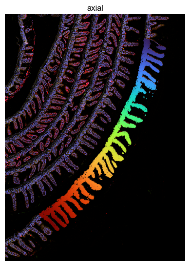
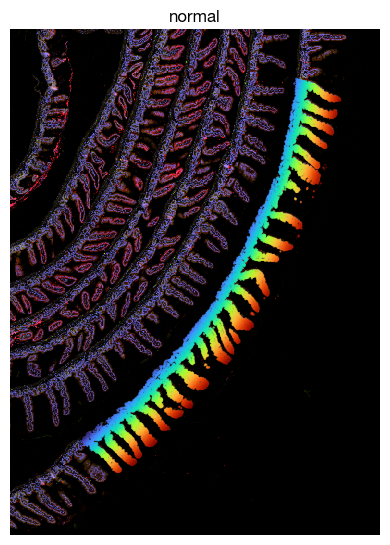
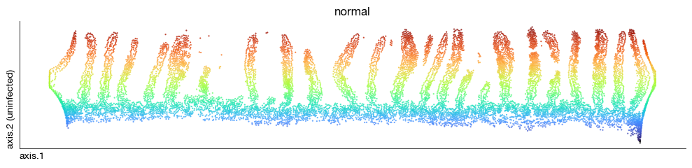
Many tissues exhibit organized spatial structures such as crypt-villus axes in the intestine, radial layers in the brain, or proximal-distal gradients in developmental systems. Quantifying gene expression and cell identity along these anatomical axes provides insights into the functional organization of tissues. This notebook demonstrates the construction of axial and normal coordinate systems for spatial data using the exprmat package. We define a tissue region of interest using a polygonal boundary, compute axial (along-tissue) and normal (cross-tissue) coordinates for each cell, and visualize molecular patterns along these axes. Distance metrics to specified tissue patches are also calculated, enabling proximity-based analysis of cell populations relative to anatomical landmarks.
[1]:
%load_ext autoreload
%autoreload 2
[2]:
import exprmat as em
em.setwd('../../../data')
ver = em.version()
[i] exprmat 0.2.66 / exprmat-db 0.2.66
[i] os: posix (linux)  platform version: 6.8.0-90-generic
[i] loaded configuration from /home/data/yangz/.exprmatrc
[i] current working directory: /home/data/yangz/packages/exprmat/data
[i] current database directory: /home/data/yangz/packages/database (0.2.66)
[i] resident memory: 777.61 MiB
[i] virtual memory: 5.95 GiB
[3]:
expm = em.load_experiment('expm/xenium')
━━━━━━━━━━━━━━━━━━━━━━━━━━ loading samples 2 / 2 (00:27 < 00:00)
[!] integrated mudata object is not generated.
[6]:
print(expm)
[!] dataset not integrated.
[*] composed of samples:
  uninfected   spatial-cell mmu    batch b1      of size 219073 × 451
  roi-villi    spatial-cell mmu    batch b1      of size 1759 × 451
[11]:
expm.spatial_cell.view('uninfected')
annotated data of size 219073 × 451
    obs : sample <cat> batch <cat> group <cat> modality <cat> taxa <cat> barcode <o> ubc <o>
          x <f64> y <f64> area <f64> x.nucleus <f64> y.nucleus <f64> area.nucleus <f64> z <f64>
          n.nucleus <f64> cid <ui32> cid.tag <ui32> segment <i64> pixellated <o> smoothened <o>
          circularity <f64>
    var : chr <cat> start <i64> end <i64> strand <cat> id <o> subtype <cat> gene <o> tlen <f64>
          cdslen <i64> assembly <cat> uid <o>
   obsm : segment <df> spatial <arr:f64(2)>
    uns : spatial
[10]:
expm.spatial_cell.summary(run_on_samples = ['uninfected'])
uninfected
├── lores  of shape 4268 ✗ 5108 ✗ 4
│       [0] nucleus   [1] membrane  [2] 18s       [3] asma-vim
├── mask  of shape 40865 ✗ 34148
├── mask-nucleus  of shape 40865 ✗ 34148
└── origin  of shape 34148 ✗ 40865 ✗ 4
        [0] nucleus   [1] membrane  [2] 18s       [3] asma-vim
Axial and normal axis#
From a thin segment of the slide (of any shape), and two user-specified points near the start and end of the segment, an central axis and its normal axis can be constructed. The following defines a region of part of the Swiss roll, in global coordinate system
[12]:
vertex = em.np.array([
    [6319.020, 4206.571],
    [6414.335, 4189.436],
    [6512.863, 4162.662],
    [6614.603, 4124.108],
    [6681.002, 4094.121],
    [6703.492, 4086.624],
    [6691.712, 3983.812],
    [6677.789, 3924.910],
    [6661.725, 3877.788],
    [6645.661, 3798.537],
    [6628.525, 3715.003],
    [6579.262, 3561.856],
    [6559.984, 3474.038],
    [6537.494, 3381.936],
    [6511.792, 3314.466],
    [6463.599, 3190.235],
    [6444.322, 3119.552],
    [6404.696, 3032.805],
    [6378.993, 2970.690],
    [6350.077, 2885.013],
    [6305.097, 2796.124],
    [6256.904, 2707.235],
    [6207.641, 2607.636],
    [6155.164, 2523.031],
    [6101.616, 2415.935],
    [6055.565, 2336.685],
    [6019.153, 2255.292],
    [5977.385, 2166.403],
    [5938.831, 2088.223],
    [5883.141, 2020.753],
    [5810.316, 1919.013],
    [5772.833, 1859.039],
    [5716.072, 1786.214],
    [5607.906, 1676.977],
    [5551.145, 1604.152],
    [5495.456, 1531.327],
    [5452.618, 1482.063],
    [5388.360, 1442.438],
    [5336.954, 1406.025],
    [5302.684, 1356.762],
    [5279.123, 1326.775],
    [5226.646, 1240.027],
    [5151.680, 1182.196],
    [5085.280, 1122.223],
    [5019.952, 1044.043],
    [4951.411, 1010.843],
    [4895.721,  977.644],
    [4872.160,  963.721],
    [4739.362, 1091.165],
    [4654.757, 1184.338],
    [4561.584, 1289.291],
    [4633.337, 1341.768],
    [4700.808, 1383.535],
    [4744.717, 1422.090],
    [4795.052, 1454.218],
    [4862.522, 1514.192],
    [4908.573, 1560.243],
    [4954.624, 1596.655],
    [5003.888, 1631.997],
    [5055.294, 1686.616],
    [5097.061, 1735.880],
    [5138.828, 1789.427],
    [5180.595, 1848.330],
    [5219.150, 1882.600],
    [5266.271, 1942.574],
    [5323.032, 1991.838],
    [5371.225, 2038.960],
    [5394.786, 2082.869],
    [5433.340, 2127.849],
    [5478.320, 2192.106],
    [5511.520, 2228.518],
    [5565.068, 2300.272],
    [5603.622, 2342.040],
    [5644.319, 2413.794],
    [5673.234, 2467.341],
    [5695.724, 2509.108],
    [5722.498, 2562.656],
    [5785.685, 2633.339],
    [5802.820, 2670.823],
    [5816.742, 2722.228],
    [5837.090, 2752.215],
    [5872.432, 2815.401],
    [5904.560, 2888.226],
    [5925.980, 2942.845],
    [5944.186, 3000.677],
    [6008.443, 3114.198],
    [6033.075, 3173.100],
    [6066.275, 3200.945],
    [6086.623, 3265.202],
    [6120.893, 3346.595],
    [6142.312, 3407.639],
    [6170.157, 3480.464],
    [6187.292, 3543.650],
    [6201.215, 3605.766],
    [6216.208, 3655.030],
    [6231.202, 3764.267],
    [6246.195, 3808.176],
    [6259.047, 3873.504],
    [6279.395, 3933.478],
    [6285.820, 4000.948],
    [6297.601, 4051.283],
    [6301.885, 4135.888],
    [6319.020, 4206.571]
])
[13]:
expm.spatial_cell.coordinates_axial_normal(
    run_on_samples = ['uninfected'],
    region_polygon = vertex.tolist(),
    starting = (6504, 4130),
    ending = (4805, 1149),
    axial_key_added = 'axial',
    normal_key_added = 'normal',
    coordinate_key_added = 'axis',
    seed_dilation_radius = 5,
    streamline_step = 0.5,
    curve_smooth_factor  = 0.0,
    n_curve_points = 500,
)
[i] rasterized region polygon into 280 x 418 mask for sample 'uninfected'
[i] solving harmonic on 23536 foreground pixels ...
[i] bicgstab did not fully converge (code -10), trying spsolve ...
[i] medial seed at xy=(169.0, 187.0), u=0.549
[i] raw streamline has 840 waypoints
[i] 207705 cells lie outside the region polygon and received NaN coordinates
Only cells within the region be assigned with an axial and normal coordinate. Other cells were set to float NaN’s
[14]:
expm.spatial_cell['uninfected'].obs[['axial', 'normal', 'x', 'y']].loc[
    ~ em.np.isnan(expm.spatial_cell['uninfected'].obs['axial']), :
]
[14]:
| axial | normal | x | y | |
|---|---|---|---|---|
| uninfected:23783 | 0.629481 | -1.670593 | 5700.353516 | 2167.714111 |
| uninfected:23784 | 0.629527 | -2.366043 | 5695.682129 | 2170.752686 |
| uninfected:23785 | 0.626580 | -3.593798 | 5693.799805 | 2185.289062 |
| uninfected:23786 | 0.625064 | -3.849591 | 5695.283691 | 2191.034668 |
| uninfected:23787 | 0.624969 | -3.071870 | 5700.606934 | 2187.780273 |
| ... | ... | ... | ... | ... |
| uninfected:218507 | 0.146003 | -16.080246 | 6278.808105 | 3701.526855 |
| uninfected:218508 | 0.146031 | -16.739316 | 6273.619141 | 3702.430664 |
| uninfected:218509 | 0.141642 | -18.692567 | 6261.741211 | 3719.874023 |
| uninfected:218510 | 0.147299 | -18.241949 | 6260.756348 | 3700.448975 |
| uninfected:218511 | 0.146028 | -18.405190 | 6260.496582 | 3704.875000 |
11368 rows × 4 columns
[15]:
fig = expm.spatial_cell.plot_spatial(
    run_on_samples = ['uninfected'],
    channels = [
        'lores/nucleus',
        'lores/membrane',
        'lores/18s',
        'lores/asma-vim'
    ],
    channel_colors = [
        "#6b6bff",
        '#ff0000',
        '#ffff00',
        '#00ff00'
    ],
    plot_embeddings = {
        'visible': True,
        'basis': 'spatial',
        'color': 'axial',
        'ticks': True,
        'cmap': 'turbo',
        'ptsize': 2,
    },
    plot_cells = {
        'visible': False,
        # plot cell boundary
        'key_boundary': 'smoothened',
        'color': 'axial',
        'subset': None,
        'alpha': 0.3,
        'filled': False,
        'palette': 'turbo',
        'legend': False,
    },
    xrange = (4000, 7000),
    yrange = (500, 4600),
    ticks = True,
    figsize = (4, 6), dpi = 100,
)
[16]:
fig = expm.spatial_cell.plot_spatial(
    run_on_samples = ['uninfected'],
    channels = [
        'lores/nucleus',
        'lores/membrane',
        'lores/18s',
        'lores/asma-vim'
    ],
    channel_colors = [
        "#6b6bff",
        '#ff0000',
        '#ffff00',
        '#00ff00'
    ],
    plot_embeddings = {
        'visible': True,
        'basis': 'spatial',
        'color': 'normal',
        'ticks': True,
        'cmap': 'turbo',
        'ptsize': 2,
        'vmin': None, 'vmax': None,
    },
    plot_cells = {
        'visible': False,
        # plot cell boundary
        'key_boundary': 'smoothened',
        'color': 'axial',
        'subset': None,
        'alpha': 0.3,
        'filled': False,
        'palette': 'turbo',
        'legend': False,
    },
    xrange = (4000, 7000),
    yrange = (500, 4600),
    ticks = True,
    figsize = (4, 6), dpi = 100,
)
[17]:
expm.spatial_cell.view('uninfected')
annotated data of size 219073 × 451
    obs : sample <cat> batch <cat> group <cat> modality <cat> taxa <cat> barcode <o> ubc <o>
          x <f64> y <f64> area <f64> x.nucleus <f64> y.nucleus <f64> area.nucleus <f64> z <f64>
          n.nucleus <f64> cid <ui32> cid.tag <ui32> segment <i64> pixellated <o> smoothened <o>
          circularity <f64> axial <f64> <f/coordinate> normal <f64> <f/coordinate>
    var : chr <cat> start <i64> end <i64> strand <cat> id <o> subtype <cat> gene <o> tlen <f64>
          cdslen <i64> assembly <cat> uid <o>
   obsm : segment <df> spatial <arr:f64(2)> axis <df> <f/coordinate:2d/embedding>
    uns : spatial
[38]:
fig = expm.spatial_cell.plot_embedding(
    run_on_samples = ['uninfected'],
    basis = 'axis', color = 'normal',
    sort = True, figsize = (10, 2.5), dpi = 100, legend = False,
    annotate_style = 'text', annotate_fontsize = 8, ptsize = 2,
    vmin = None, vmax = None
)
Distance metrics to patches#
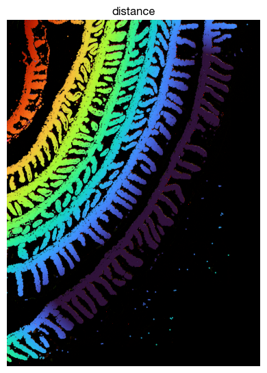
Distance metrics can be derived to serve as a proximal-distal axis to regions of interest.
[33]:
expm.spatial_cell.coordinates_proximal_distal(
    run_on_samples = ['uninfected'],
    region_polygons = [vertex.tolist()],
    key_added = 'distance'
)
[i] computing proximal-distal distances for 219073 cells against 1 polygon(s) in sample 'uninfected'
[i] proximal-distal distances written to obs['distance']
[39]:
s = 'uninfected'
fig = expm.spatial_cell.plot_spatial(
    run_on_samples = [s],
    channels = [
        'lores/nucleus',
        'lores/membrane',
        'lores/18s',
        'lores/asma-vim'
    ],
    channel_colors = [
        "#6b6bff",
        '#ff0000',
        '#ffff00',
        '#00ff00'
    ],
    plot_embeddings = {
        'visible': True,
        'basis': 'spatial',
        'color': 'distance',
        'ticks': True,
        'cmap': 'turbo',
        'cmap_lower': None,
        'ptsize': 2,
    },
    plot_cells = {
        'visible': False,
        # plot cell boundary
        'key_boundary': 'smoothened',
        'color': 'axial',
        'subset': None,
        'alpha': 0.3,
        'filled': False,
        'palette': 'turbo',
        'legend': False,
    },
    xrange = (4000, 7000),
    yrange = (500, 4600),
    ticks = True,
    figsize = (4, 6), dpi = 100,
)
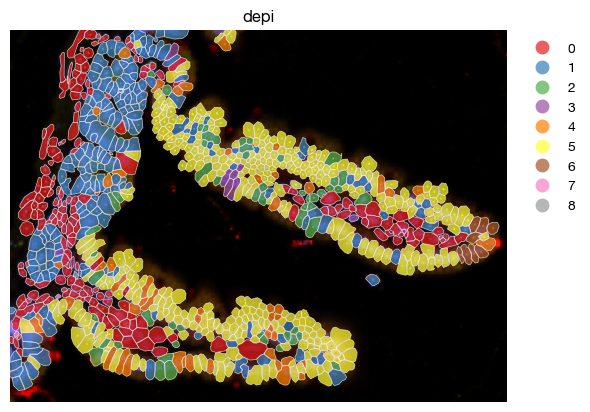
Minimal distance to a subset of cells#
Similar nearest neighbor distance can be derived from a subset of target cells, other than geometric shapes.
[ ]:
expm.spatial_cell.coordinates_minimal_distance(
    run_on_samples = ['uninfected'],
    cluster_key = 'leiden',
    cluster_values = ['5'],
    key_added = 'depi'
)
[23]:
s = 'uninfected'
fig = expm.spatial_cell.plot_spatial(
    run_on_samples = [s],
    channels = [
        'lores/nucleus',
        'lores/membrane',
        'lores/18s',
        'lores/asma-vim'
    ],
    channel_colors = [
        "#6b6bff",
        '#ff0000',
        '#ffff00',
        '#00ff00'
    ],
    plot_embeddings = {
        'visible': True,
        'basis': 'spatial',
        'color': 'depi',
        'ticks': True,
        'cmap': 'turbo',
        'cmap_lower': None,
        'ptsize': 2,
        'vmax': 100
    },
    plot_cells = {
        'visible': True,
        # plot cell boundary
        'key_boundary': 'smoothened',
        'color': 'leiden',
        'subset': None,
        'alpha': 0.7,
        'filled': True,
        'palette': 'set1',
        'legend': True,
        'vmax': 100
    },
    xrange = (5900, 6300),
    yrange = (2700, 3000),
    ticks = True,
    figsize = (6, 6), dpi = 100,
)
[ ]:
s = 'uninfected'
fig = expm.spatial_cell.plot_spatial(
    run_on_samples = [s],
    channels = [
        'lores/nucleus',
        'lores/membrane',
        'lores/18s',
        'lores/asma-vim'
    ],
    channel_colors = [
        "#6b6bff",
        '#ff0000',
        '#ffff00',
        '#00ff00'
    ],
    plot_embeddings = {
        'visible': True,
        'basis': 'spatial',
        'color': 'depi',
        'ticks': True,
        'cmap': 'turbo',
        'cmap_lower': None,
        'ptsize': 2,
        'vmax': 100
    },
    plot_cells = {
        'visible': True,
        # plot cell boundary
        'key_boundary': 'smoothened',
        'color': 'depi',
        'subset': None,
        'alpha': 0.7,
        'filled': True,
        'palette': 'set1',
        'legend': True,
        'vmax': 100
    },
    xrange = (5900, 6300),
    yrange = (2700, 3000),
    ticks = True,
    figsize = (6, 6), dpi = 100,
)
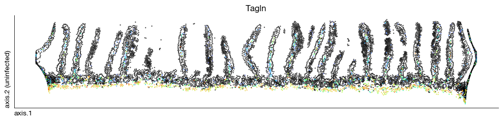
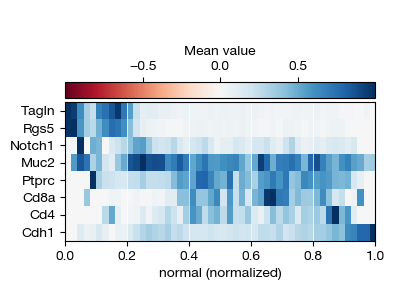
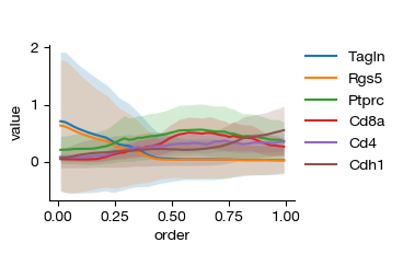
Gene expression change along axis#
You may trace gene expression along axis. Note that pseudotemporal axis and spatial axis share the same set of plotting functions since they were exactly one thing logically.
[ ]:
expm.spatial_cell.log_normalize(
    run_on_samples = ['uninfected'],
    key_norm = 'norm',
    key_lognorm = 'lognorm'
)
[68]:
fig = expm.spatial_cell.plot_embedding(
    run_on_samples = ['uninfected'],
    basis = 'axis', color = 'Tagln',
    sort = True, figsize = (10, 2.5), dpi = 100, legend = False,
    annotate_style = 'text', annotate_fontsize = 8, ptsize = 2,
    vmin = None, vmax = None
)
[89]:
fig = expm.spatial_cell.plot_variable_order(
    run_on_samples = ['uninfected'],
    features = ['Tagln', 'Rgs5', 'Notch1', 'Muc2', 'Ptprc', 'Cd8a', 'Cd4', 'Cdh1'],
    ordering = 'normal',
    min_ordering = None,
    max_ordering = None,
    cmap = 'rdbu',
    bins = 50,
    style = 'matrix',
    layer = 'X',
    figsize = (4, 3),
)
[ ]:
fig = expm.spatial_cell.plot_variable_order(
    run_on_samples = ['uninfected'],
    features = ['Tagln', 'Rgs5', 'Ptprc', 'Cd8a', 'Cd4', 'Cdh1'],
    ordering = 'normal',
    min_ordering = None,
    max_ordering = None,
    cmap = 'rdbu',
    bins = 50,
    style = 'line',
    layer = 'X',
    figsize = (4, 2.5),
)
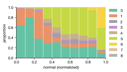
Proportion change along axis#
Tracking categorical compositions other than continuous variable is also available.
[93]:
expm.spatial_cell.select_hvg(
    run_on_samples = [s],
    key_lognorm = 'lognorm',
    method = 'vst',
    dest = 'vst',
    n_top_genes = 200
)
[94]:
expm.spatial_cell.scale_pca(
    run_on_samples = [s],
    hvg = 'vst.hvg',
    key_lognorm = 'lognorm',
    key_scaled = 'scaled',
    key_added = 'pca', n_comps = 35,
    keep_sparse = True,
    random_state = 42,
    svd_solver = 'arpack'
)
[95]:
expm.spatial_cell.knn(
    run_on_samples = [s],
    use_rep = 'pca',
    n_comps = None,
    n_neighbors = 30,
    knn = True,
    method = "umap",
    transformer = None,
    metric = "euclidean",
    metric_kwds = {},
    random_state = 42,
    key_added = 'neighbors',
    use_gpu = True
)
[106]:
expm.spatial_cell.leiden(
    run_on_samples = [s],
    resolution = 0.1,
    restrict_to = None,
    random_state = 42,
    key_added = 'leiden',
    adjacency = None,
    directed = None,
    use_weights = True,
    n_iterations = 2,
    partition_type = None,
    neighbors_key = None,
    obsp = None,
    flavor = 'igraph',
    use_gpu = True
)
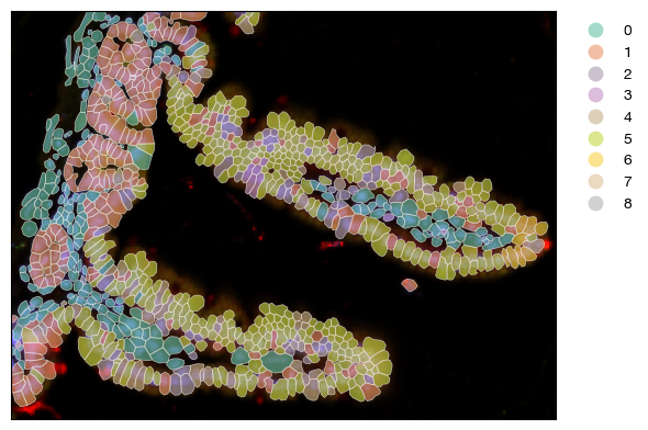
[14]:
fig = expm.spatial_cell.plot_spatial(
    run_on_samples = ['uninfected'],
    channels = [
        'lores/nucleus',
        'lores/membrane',
        'lores/18s',
        'lores/asma-vim'
    ],
    channel_colors = [
        "#6b6bff",
        '#ff0000',
        '#ffff00',
        '#00ff00'
    ],
    plot_embeddings = { 'visible': False, },
    plot_cells = {
        'visible': True,
        # plot cell boundary
        'key_boundary': 'smoothened',
        'color': 'leiden',
        'subset': None,
        'alpha': 0.6,
        'linewidth': 0.5,
        'filled': True,
        'palette': 'set2',
        'legend': True,
    },
    xrange = (5900, 6300),
    yrange = (2700, 3000),
    ticks = False,
    figsize = (6, 6), dpi = 100,
)
[12]:
fig = expm.spatial_cell.plot_proportion_order(
    run_on_samples = ['uninfected'],
    category = 'leiden',
    ordering = 'normal',
    min_ordering = None,
    max_ordering = None,
    cmap = 'set2',
    bins = 10,
    figsize = (4, 2.5),
)
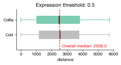
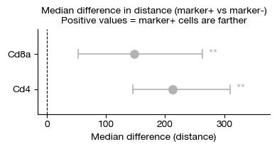
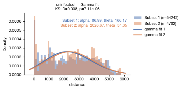
Subtype distance comparison#
We have provided several statistical comparison tools for quick assessment of distance variation. You may implement yours easily since you can get the proximity axis directly from .obs with custom statistical methods.
[24]:
fig = expm.spatial_cell.plot_proximity_markers(
    run_on_samples = ['uninfected'],
    features = ['Cd8a', 'Cd4'],
    proximity = 'distance',
    min_proximity = 0,
    max_proximity = 500,
    feature_threshold = 0.5,
    cmap = 'set2',
    layer = 'X',
    subset = lambda x: x['leiden'] == '0',
    figsize = (4, 2.2),
)
[27]:
fig = expm.spatial_cell.plot_proximity_difference(
    run_on_samples = ['uninfected'],
    features = ['Cd8a', 'Cd4'],
    proximity = 'distance',
    min_proximity = 0,
    max_proximity = 500,
    n_iterations = 1000,
    feature_threshold = 0.5,
    cmap = 'set2',
    layer = 'X',
    subset = lambda x: x['leiden'] == '0',
    figsize = (4, 2.2),
)
[16]:
fig = expm.spatial_cell.plot_distance_distribution(
    run_on_samples = ['uninfected'],
    ordering = 'distance',
    subset1 = lambda x: x['leiden'] == '5',
    subset2 = lambda x: x['leiden'] == '6',
    fit = 'gamma',
    bins = 50,
    figsize = (6, 3),
    dpi = 100,
)
[46]:
expm.save()
[i] saving individual samples. (pass `save_samples = False` to skip)
━━━━━━━━━━━━━━━━━━━━━━━ modality [spatial-cell] 2 / 2 (00:16 < 00:00)