Statistics

We introduce several basic utility functions for summarizing and computing statistics on sparse matrices.

%load_ext autoreload
%autoreload 2

import exprmat as em
# set working directory
em.setwd('../../../data')
ver = em.version()

[i] exprmat 0.2.66 / exprmat-db 0.2.66
[i] os: posix (linux)  platform version: 6.8.0-90-generic
[i] loaded configuration from /home/data/yangz/.exprmatrc
[i] current working directory: /home/data/yangz/packages/exprmat/data
[i] current database directory: /home/data/yangz/packages/database (0.2.66)
[i] resident memory: 778.73 MiB
[i] virtual memory: 5.95 GiB

expm = em.load_experiment('expm/scrna', load_subset = 'mono-neutro')

   ━━━━━━━━━━━━━━━━━━━━━━━━━━ loading samples          3 / 3     (00:03 < 00:00)

print(expm)

annotated data of size 9754 × 19651
subset mono-neutro of size 9754 × 19651
contains modalities: rna

 modality [rna]
    obs : sample <cat> <c/sample> batch <cat> <c/batch> group <cat> <c> modality <cat> <c/modality>
          taxa <cat> <c/taxa> barcode <o> <o> ubc <o> <o> n.umi <f64> <i> n.genes <i64> <i>
          n.mito <f64> <f> n.ribo <f64> <f> pct.mito <f64> <f> pct.ribo <f64> <f>
          filter <bool> <bool> score.doublet <f64> <f> score.doublet.se <f64> <f>
          is.doublet <bool> <bool> qc <bool> <bool/qc> leiden <cat> <c> sc3.5 <cat> <c>
          sc3.10 <cat> <c> sc3.20 <cat> <c> sc3.30 <cat> <c> cell.type <cat> <c>
    var : chr <cat> <c/chromosome> start <i64> <i> end <i64> <i> strand <cat> <c/strand> id <o> <o>
          subtype <cat> <c/gsubtype> gene <cat> <o/gene> tlen <f64> <i/tlen> cdslen <i64> <i/cdslen>
          assembly <cat> <c> uid <o> <o/ugene> vst.hvg <bool> <bool/hvg> vst.all.means <f64> <f>
          vst.all.vars <f64> <f> vst.all.vars.norm <f64> <f> vst.all.hvg.rank <f32> <f>
          vst.all.hvg <bool> <bool>
 layers : counts <f32> <i/counts> norm <f32> <f>
   obsm : cnmf.10 <df> <f/embedding/usage> harmony <arr:f32(35)> <f> knn <arr:i32(100)> <i/knni>
          knn.d <arr:f32(100)> <f/knnd> pca <arr:f64(35)> <f/embedding/pca>
          umap <arr:f32(2)> <f/embedding>
   varm : cnmf.10 <arr:f64(10)> <f/weights> cnmf.coef.10 <arr:f64(10)> <f/usage-coef>
          pca <arr:f64(35)> <f/weights>
   obsp : connectivities <csr:f32> <f/connectivity> distances <csr:f32> <f/distance>
    uns : cell.type.colors cell.type_colors cnmf <cnmf> cnmf.args <o>
          cnmf.density.10 <cnmf-density> cnmf.dist.10 <f/connectivity> cnmf.stats <cnmf-stats>
          commands <system> leiden <o> leiden.colors <o> markers <markers> neighbors <knn>
          pca <dict> sc3.10.colors <o> sc3.20.colors <o> sc3.30.colors <o> sc3.5.colors <o>
          slots <system> umap <o>

[*] composed of samples:
  distal   rna   mmu    batch b1      of size 6451 × 21689
  niche    rna   mmu    batch b2      of size 3656 × 21970
  normal   rna   mmu    batch b3      of size 4537 × 21917

Cluster proportion statistics

Compute the proportions of categorical variables across dataset rows (cells). The major parameter specifies the primary grouping variable, while minor specifies the categorical variable for which proportions are calculated.

expm.rna.proportion(
    major = 'sample', minor = 'cell.type',
    normalize = 'index'
)['integrated']

cell.type	DCp	MDP	MM	Mo	Neu	Prog	iMac
sample
distal	0.023297	0.062052	0.080421	0.035842	0.774194	0.023970	0.000224
niche	0.001878	0.160345	0.079985	0.088246	0.563275	0.024784	0.081487
normal	0.065855	0.159878	0.051389	0.031976	0.666159	0.023601	0.001142

Gaussian kernel density estimation

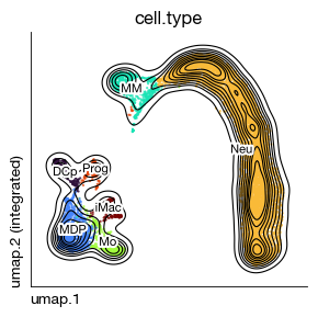
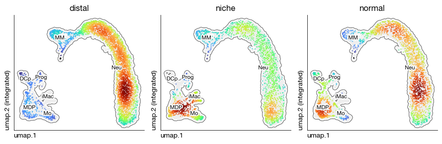
Given a low-dimensional representation, we can compute the density of the scatter point distribution to visualize how cells are concentrated in different regions of the embedding space.

fig = expm.rna.plot_embedding(
    basis = 'umap', color = 'cell.type',
    figsize = (3, 3), dpi = 100, legend_col = 2, legend = False,
    ptsize = 2, annotate_style = 'text', annotate_fontsize = 8, contour_plot = True
)

expm.rna.kde(
    basis = "umap",
    groupby = "sample",
    key_added = "kde.umap",
    components = "1,2"
)

kde = expm.rna.plot_kde(
    basis = 'umap', kde = 'kde.umap', grouping_key = 'sample',
    background = 'cell.type', annotate = True, annotate_fontsize = 8, ptsize = 2,
    figsize = (9, 3), dpi = 100, groups = None, ncols = 3, cmap = 'turbo'
)

Summary statistics

The summary function creates a three-dimensional table using the on, across, and split parameters. Each cell value in the table is computed from the data, orient, and method parameters. The returned object is an AnnData structure where rows correspond to on, columns correspond to across, and layers contain each split.

When orient is set to 'obs', the on, across, and split parameters must be column names in the obs table. Similarly, when orient is set to 'var', these must be column names in the var table. Specific rows or columns are selected by the three filter conditions, and the method function is applied to produce the cell values of the three-dimensional table. If the filtered result is an empty set, the corresponding cell is NaN.

When method is set to the special method n, it returns the count of observations (rows or columns, not the count of values within the statistical range).

adata = expm.rna.summary(
    data = 'X', method = 'n', method_args = {},
    orient = 'obs', on = 'sample',
    across = 'cell.type', split = 'sample',
    attached_metadata_on = None, attached_metadata_across = None,
    attach_method_on = 'first', attach_method_across = 'first'
)['integrated']

em.pd.DataFrame(
    adata.layers['niche'],
    index = adata.obs_names,
    columns = adata.var_names
)

	Neu	MDP	MM	Mo	DCp	Prog	iMac
distal	NaN	NaN	NaN	NaN	NaN	NaN	NaN
niche	1500.0	427.0	213.0	235.0	5.0	66.0	217.0
normal	NaN	NaN	NaN	NaN	NaN	NaN	NaN

Aggregate statistics

The aggregate function collapses the original data table along rows or columns, applying a specified method (such as sum or mean) to groups defined by observation or variable keys.

adata = expm.rna.aggregate(
    data = 'counts', method = 'sum', method_args = {},
    obs_key = 'sample', var_key = None
)['integrated']

em.pd.DataFrame(
    adata.X,
    index = adata.obs_names,
    columns = adata.var['gene']
).iloc[:, 0:10]

gene	Bzw1	Ppp1r9b	Samd14	Clk1	Pdk2	Itga3	Ppil3	Tac4	Kat7	Gm11520
distal	4153.0	1685.0	29.0	6723.0	54.0	0.0	456.0	2.0	1604.0	144.0
niche	3908.0	2584.0	42.0	4752.0	46.0	11.0	442.0	6.0	1415.0	110.0
normal	3470.0	1561.0	21.0	4831.0	72.0	1.0	446.0	8.0	1292.0	129.0

Pseudobulking

Pseudobulking merges cells from a specified category by counts, and continue the analysis normalization as if they were coming from bulk dataset.

expm.rna.annotate_paste(
    froms = ['sample', 'cell.type'],
    into = 'psbulk',
    slot = 'rna',
    sep = ':'
)

psbulk
distal:Neu     3456
normal:Neu     1750
niche:Neu      1500
niche:MDP       427
normal:MDP      420
distal:MM       359
distal:MDP      277
niche:Mo        235
niche:iMac      217
niche:MM        213
normal:DCp      173
distal:Mo       160
normal:MM       135
distal:Prog     107
distal:DCp      104
normal:Mo        84
niche:Prog       66
normal:Prog      62
niche:DCp         5
normal:iMac       3
distal:iMac       1
Name: count, dtype: int64

expm.rna.pseudobulk(
    obs_key = 'psbulk',
    sample_added = 'psbulk',
    obs_metadata = ['cell.type', 'sample', 'group'],
    merge_obs_metadata = 'mode'
)

[i] created subset [psbulk] from sample [integrated]

print(expm)

annotated data of size 9754 × 19651
subset mono-neutro of size 9754 × 19651
contains modalities: rna

 modality [rna]
    obs : sample <cat> <c/sample> batch <cat> <c/batch> group <cat> <c> modality <cat> <c/modality>
          taxa <cat> <c/taxa> barcode <o> <o> ubc <o> <o> n.umi <f64> <i> n.genes <i64> <i>
          n.mito <f64> <f> n.ribo <f64> <f> pct.mito <f64> <f> pct.ribo <f64> <f>
          filter <bool> <bool> score.doublet <f64> <f> score.doublet.se <f64> <f>
          is.doublet <bool> <bool> qc <bool> <bool/qc> leiden <cat> <c> sc3.5 <cat> <c>
          sc3.10 <cat> <c> sc3.20 <cat> <c> sc3.30 <cat> <c> cell.type <cat> <c>
          kde.umap <f64> <f/kde> psbulk <cat>
    var : chr <cat> <c/chromosome> start <i64> <i> end <i64> <i> strand <cat> <c/strand> id <o> <o>
          subtype <cat> <c/gsubtype> gene <cat> <o/gene> tlen <f64> <i/tlen> cdslen <i64> <i/cdslen>
          assembly <cat> <c> uid <o> <o/ugene> vst.hvg <bool> <bool/hvg> vst.all.means <f64> <f>
          vst.all.vars <f64> <f> vst.all.vars.norm <f64> <f> vst.all.hvg.rank <f32> <f>
          vst.all.hvg <bool> <bool>
 layers : counts <f32> <i/counts> norm <f32> <f>
   obsm : cnmf.10 <df> <f/embedding/usage> harmony <arr:f32(35)> <f> knn <arr:i32(100)> <i/knni>
          knn.d <arr:f32(100)> <f/knnd> pca <arr:f64(35)> <f/embedding/pca>
          umap <arr:f32(2)> <f/embedding>
   varm : cnmf.10 <arr:f64(10)> <f/weights> cnmf.coef.10 <arr:f64(10)> <f/usage-coef>
          pca <arr:f64(35)> <f/weights>
   obsp : connectivities <csr:f32> <f/connectivity> distances <csr:f32> <f/distance>
    uns : cell.type.colors cell.type_colors cnmf <cnmf> cnmf.args <o>
          cnmf.density.10 <cnmf-density> cnmf.dist.10 <f/connectivity> cnmf.stats <cnmf-stats>
          commands <system> leiden <o> leiden.colors <o> markers <markers> neighbors <knn>
          pca <dict> sc3.10.colors <o> sc3.20.colors <o> sc3.30.colors <o> sc3.5.colors <o>
          slots <system> umap <o> kde.umap <kde-stats>

[*] composed of samples:
  distal   rna   mmu    batch b1        of size 6451 × 21689
  niche    rna   mmu    batch b2        of size 3656 × 21970
  normal   rna   mmu    batch b3        of size 4537 × 21917
  psbulk   rna   autogen   batch autogen   of size 21 × 19651

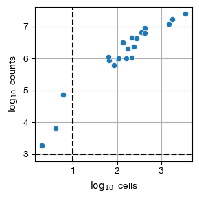
fig = expm.rna.plot_pseudobulk_samples(
    run_on_samples = ['psbulk'],
    groupby = None, figsize = (3, 3),
    min_cells = 10, min_counts = 1000,
    log = True,
)

expm.rna.filter_pseudobulk_samples(
    run_on_samples = ['psbulk'],
    min_cells = 10, min_counts = 1000,
)

expm.rna.view('psbulk')

annotated data of size 18 × 19651
    obs : cell.type <o> <c> sample <o> <c/sample> group <o> <c> counts <f32> <f> cells <i64> <i>
    var : chr <cat> <c/chromosome> start <i64> <i> end <i64> <i> strand <cat> <c/strand> id <o> <o>
          subtype <cat> <c/gsubtype> gene <cat> <o/gene> tlen <f64> <i/tlen> cdslen <i64> <i/cdslen>
          assembly <cat> <c> uid <o> <o/ugene> vst.hvg <bool> <bool/hvg> vst.all.means <f64> <f>
          vst.all.vars <f64> <f> vst.all.vars.norm <f64> <f> vst.all.hvg.rank <f32> <f>
          vst.all.hvg <bool> <bool>
 layers : proportions <f64> <f/proportions>
    uns : slots <system> commands <system>

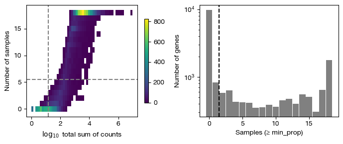
fig = expm.rna.plot_pseudobulk_features(
    run_on_samples = ['psbulk'],
    group = 'group',
    lib_size = None,
    min_count = 10,
    min_total_count = 15,
    large_n = 10,
    min_sample_prop = 0.7,
    cmap = 'viridis',
    min_cell_prop = 0.2,
    min_samples = 2,
    figsize = (7, 3),
    dpi = 100
)

expm.rna.filter_pseudobulk_features(
    run_on_samples = ['psbulk'],
    group = 'group',
    lib_size = None,
    min_count = 10,
    min_total_count = 15,
    large_n = 10,
    min_sample_prop = 0.7,
    min_cell_prop = 0.2,
    min_samples = 2
)

expm.save()

[i] main dataset write to expm/scrna/subsets/mono-neutro.h5mu
[i] saving individual samples. (pass `save_samples = False` to skip)

   ━━━━━━━━━━━━━━━━━━━━━━━━━━ modality [rna]           4 / 4     (00:01 < 00:00)