Bin-based Spatial Profiling

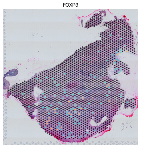
This notebook demonstrates the analysis of bin-based spatial transcriptomics data using the exprmat package, focusing on the 10x Visium platform. Visium technology captures gene expression across spatially barcoded spots arranged on a grid, where each spot typically spans multiple cells. We work through the complete workflow from metadata specification and experiment construction, through spatial visualization of gene expression on the tissue image, log normalization and dimensionality reduction, to clustering and the visualization of cluster assignments in both UMAP space and the original tissue coordinates. Integration of clusters across multiple slides is also discussed.

%load_ext autoreload
%autoreload 2

import exprmat as em
em.setwd('../../../data')
ver = em.version()

[i] exprmat 0.2.66 / exprmat-db 0.2.66
[i] os: posix (linux)  platform version: 6.8.0-90-generic
[i] loaded configuration from /home/data/yangz/.exprmatrc
[i] current working directory: /home/data/yangz/packages/exprmat/data
[i] current database directory: /home/data/yangz/packages/database (0.2.66)
[i] resident memory: 777.60 MiB
[i] virtual memory: 5.95 GiB

samples = ['p1-t4', 'p1-t5', 'p1-t7', 'p1-t10', 'p2-t1', 'p2-t2', 'p2-t5', 'p2-t6']
meta = em.metadata(
    locations = ['visium/' + x for x in samples],
    modality = ['visium'] * 8, # for visium v1 data.
    default_taxa = ['hsa'] * 8,
    names = samples,
    batches = ['b' + str(x + 1) for x in range(len(samples))],
    groups = ['p1'] * 4 + ['p2'] * 4
)

meta.dataframe

	location	sample	batch	group	modality	taxa
0	visium/p1-t4	p1-t4	b1	p1	visium	hsa
1	visium/p1-t5	p1-t5	b2	p1	visium	hsa
2	visium/p1-t7	p1-t7	b3	p1	visium	hsa
3	visium/p1-t10	p1-t10	b4	p1	visium	hsa
4	visium/p2-t1	p2-t1	b5	p2	visium	hsa
5	visium/p2-t2	p2-t2	b6	p2	visium	hsa
6	visium/p2-t5	p2-t5	b7	p2	visium	hsa
7	visium/p2-t6	p2-t6	b8	p2	visium	hsa

expm = em.experiment(meta, dump = 'expm/visium')

[i] reading sample p1-t4 [visium] ...
[i] 939 genes (out of 36601) not in the reference gene list.
[i] total 35662 genes mapped. 35554 unique genes.
[i] reading sample p1-t5 [visium] ...
[i] 939 genes (out of 36601) not in the reference gene list.
[i] total 35662 genes mapped. 35554 unique genes.
[i] reading sample p1-t7 [visium] ...
[i] 939 genes (out of 36601) not in the reference gene list.
[i] total 35662 genes mapped. 35554 unique genes.
[i] reading sample p1-t10 [visium] ...
[i] 939 genes (out of 36601) not in the reference gene list.
[i] total 35662 genes mapped. 35554 unique genes.
[i] reading sample p2-t1 [visium] ...
[i] 939 genes (out of 36601) not in the reference gene list.
[i] total 35662 genes mapped. 35554 unique genes.
[i] reading sample p2-t2 [visium] ...
[i] 939 genes (out of 36601) not in the reference gene list.
[i] total 35662 genes mapped. 35554 unique genes.
[i] reading sample p2-t5 [visium] ...
[i] 939 genes (out of 36601) not in the reference gene list.
[i] total 35662 genes mapped. 35554 unique genes.
[i] reading sample p2-t6 [visium] ...
[i] 939 genes (out of 36601) not in the reference gene list.
[i] total 35662 genes mapped. 35554 unique genes.

print(expm)

[!] dataset not integrated.
[*] composed of samples:
  p1-t4    spatial-bin hsa    batch b1      of size 1155 × 35554
  p1-t5    spatial-bin hsa    batch b2      of size 1726 × 35554
  p1-t7    spatial-bin hsa    batch b3      of size 1191 × 35554
  p1-t10   spatial-bin hsa    batch b4      of size 1522 × 35554
  p2-t1    spatial-bin hsa    batch b5      of size 2197 × 35554
  p2-t2    spatial-bin hsa    batch b6      of size 1853 × 35554
  p2-t5    spatial-bin hsa    batch b7      of size 1470 × 35554
  p2-t6    spatial-bin hsa    batch b8      of size 924 × 35554

s = 'p1-t5'

fig = expm.spatial_bin.plot_spatial(
    run_on_samples = [s],
    channels = ['hires/r', 'hires/g', 'hires/b'],
    plot_embeddings = {
        'visible': True,
        'basis': 'spatial',
        'color': 'FOXP3'
    },
    xrange = (300, 4200),
    yrange = (300, 4200),
    figsize = (5, 5)
)

expm.spatial_bin.summary(run_on_samples = [s])

p1-t5
└── hires  of shape 1946 ✗ 2000 ✗ 3
        [0] r  [1] g  [2] b

Integration and clustering

Now we merge all Visium samples into a single integrated object and perform standard single-cell-style processing on the spot-level expression matrix. The spots are treated as independent observations, and we apply log-normalization, highly variable gene selection, PCA, KNN graph construction, Leiden clustering, and UMAP embedding to identify spatially coherent transcriptional programs across the tissue sections.

expm.merge()

Merge all per-sample Visium objects into a single MuData using an outer join. After merging, we can proceed with joint normalization and clustering across all slides.

print(expm)

annotated data of size 12038 × 35554
integrated dataset of size 12038 × 35554
contains modalities: spatial-bin

 modality [spatial-bin]
    obs : sample <cat> batch <o> group <o> modality <o> taxa <o> barcode <o> ubc <o>
          in.tissue <i64> row <i64> col <i64> y <i64> x <i64>
    var : chr <o> start <i64> end <i64> strand <o> id <o> subtype <o> gene <o> tlen <f64>
          cdslen <i64> assembly <o> uid <o>
   obsm : spatial <arr:i64(2)>
    uns : spatial

[*] composed of samples:
  p1-t4    spatial-bin hsa    batch b1      of size 1155 × 35554
  p1-t5    spatial-bin hsa    batch b2      of size 1726 × 35554
  p1-t7    spatial-bin hsa    batch b3      of size 1191 × 35554
  p1-t10   spatial-bin hsa    batch b4      of size 1522 × 35554
  p2-t1    spatial-bin hsa    batch b5      of size 2197 × 35554
  p2-t2    spatial-bin hsa    batch b6      of size 1853 × 35554
  p2-t5    spatial-bin hsa    batch b7      of size 1470 × 35554
  p2-t6    spatial-bin hsa    batch b8      of size 924 × 35554

expm.spatial_bin.log_normalize(
    run_on_samples = True,
    key_norm = 'norm',
    key_lognorm = 'lognorm'
)

Apply log-normalization to the merged count matrix. Each spot’s raw counts are normalized by library size and log-transformed to stabilize variance across the dynamic range of expression values. This is a prerequisite for HVG selection and PCA.

expm.spatial_bin.select_hvg(
    run_on_samples = True,
    key_lognorm = 'lognorm',
    method = 'vst',
    dest = 'vst',
    n_top_genes = 800
)

Select the top 800 highly variable genes using the VST method. For spatial data, we typically select fewer HVGs than for scRNA-seq (800 vs 2000) because spot-level measurements average over multiple cells, reducing gene-level heterogeneity, and the spatial patterns of interest are often driven by a more focused set of genes.

expm.spatial_bin.scale_pca(
    run_on_samples = True,
    hvg = 'vst.hvg',
    key_lognorm = 'lognorm',
    key_scaled = 'scaled',
    key_added = 'pca', n_comps = 35,
    keep_sparse = False,
    random_state = 42,
    svd_solver = 'arpack'
)

Scale the expression data to unit variance and compute PCA on the HVG subset. The PCA provides a low-dimensional representation of the major expression variation across spots, which serves as input for both neighbor graph construction and downstream spatial domain identification.

expm.spatial_bin.knn(
    run_on_samples = True,
    use_rep = 'pca',
    n_comps = None,
    n_neighbors = 30,
    knn = True,
    method = "umap",
    transformer = None,
    metric = "cosine",
    metric_kwds = {},
    random_state = 42,
    key_added = 'neighbors'
)

Build a KNN graph on the PCA embedding using cosine distance. This graph captures transcriptional similarity between spots, enabling graph-based clustering and visualization.

expm.spatial_bin.leiden(
    run_on_samples = True,
    resolution = 0.5,
    restrict_to = None,
    random_state = 42,
    key_added = 'leiden',
    adjacency = None,
    directed = None,
    use_weights = True,
    n_iterations = 2,
    partition_type = None,
    neighbors_key = None,
    obsp = None,
    flavor = 'igraph',
    use_gpu = True
)

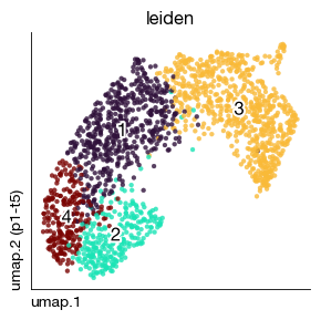
Apply the Leiden clustering algorithm to the KNN graph to partition spots into discrete clusters based on their transcriptional similarity. These clusters represent regions with shared gene expression programs and can be visualized directly on the tissue slide.

expm.spatial_bin.umap(
    run_on_samples = True,
    min_dist = 0.5,
    spread = 1,
    n_components = 2,
    maxiter = None,
    alpha = 1,
    gamma = 1,
    negative_sample_rate = 5,
    init_pos = "spectral",
    random_state = 42,
    a = None, b = None,
    key_added = 'umap',
    neighbors_key = "neighbors"
)

Compute the UMAP embedding for visualizing the spot clusters in a 2D non-linear projection. This helps assess cluster separation and identify transitional spot populations.

fig = expm.spatial_bin.plot_embedding(
    run_on_samples = [s],
    basis = 'umap', color = 'leiden',
    sort = True, figsize = (3, 3), dpi = 100, legend = False
)

fig = expm.spatial_bin.plot_spatial(
    run_on_samples = [s],
    channels = ['hires/r', 'hires/g', 'hires/b'],
    plot_embeddings = {
        'visible': True,
        'basis': 'spatial',
        'color': 'leiden',
    },
    figsize = (5.4, 5)
)

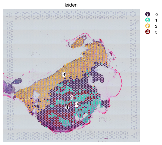
At present, leiden clusters are calculated per-slide. For integration of uniformed clusters, you may choose to do the integration (e.g. Harmony) like single cell data, or to use spatial domain identification algorithms as tutorial f1 explains.

expm.save()

[i] main dataset write to expm/visium/integrated.h5mu
[i] saving individual samples. (pass `save_samples = False` to skip)

   ━━━━━━━━━━━━━━━━━━━━━━━━ modality [spatial-bin]     8 / 8     (00:04 < 00:00)