Clustering and Annotation#

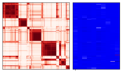
This notebook demonstrates the clustering and annotation of single-cell RNA-seq data using the exprmat package, building on the integrated dataset from the previous tutorial. After dataset creation and batch correction, we apply Leiden clustering to identify cellular subpopulations, followed by multiple complementary approaches for cluster characterization. Consensus non-negative matrix factorization (cNMF) is used to decompose expression patterns into interpretable metaprogram modules. Manual annotation based on canonical marker gene expression is performed to assign cell type identities to each cluster, and differential marker analysis validates the annotations. Finally, cell type proportions across samples are examined to compare compositional differences between experimental conditions.

[1]:

%load_ext autoreload
%autoreload 2

[2]:

import exprmat as em
# set working directory
em.setwd('../../../data')
ver = em.version()

[i] exprmat 0.2.66 / exprmat-db 0.2.66
[i] os: posix (linux)  platform version: 6.8.0-90-generic
[i] loaded configuration from /home/data/yangz/.exprmatrc
[i] current working directory: /home/data/yangz/packages/exprmat/data
[i] current database directory: /home/data/yangz/packages/database (0.2.66)
[i] resident memory: 775.91 MiB
[i] virtual memory: 5.95 GiB

[12]:

expm = em.load_experiment('expm/scrna')

   ━━━━━━━━━━━━━━━━━━━━━━━━━━ loading samples          3 / 3     (00:05 < 00:00)

[4]:

print(expm)

annotated data of size 13015 × 19651
integrated dataset of size 13015 × 19651
contains modalities: rna

 modality [rna]
    obs : sample <cat> <c/sample> batch <cat> <c/batch> group <cat> <c> modality <cat> <c/modality>
          taxa <cat> <c/taxa> barcode <o> <o> ubc <o> <o> n.umi <f64> <i> n.genes <i64> <i>
          n.mito <f64> <f> n.ribo <f64> <f> pct.mito <f64> <f> pct.ribo <f64> <f>
          filter <bool> <bool> score.doublet <f64> <f> score.doublet.se <f64> <f>
          is.doublet <bool> <bool> qc <bool> <bool/qc> leiden <cat> <c>
    var : chr <cat> <c/chromosome> start <i64> <i> end <i64> <i> strand <cat> <c/strand> id <o> <o>
          subtype <cat> <c/gsubtype> gene <cat> <o/gene> tlen <f64> <i/tlen> cdslen <i64> <i/cdslen>
          assembly <cat> <c> uid <o> <o/ugene> vst.hvg <bool> <bool/hvg> vst.all.means <f64>
          vst.all.vars <f64> vst.all.vars.norm <f64> vst.all.hvg.rank <f32> vst.all.hvg <bool>
 layers : counts <f32> <i/counts>
   obsm : harmony <arr:f32(35)> knn <arr:i32(35)> knn.d <arr:f32(35)>
          pca <arr:f64(35)> <f/embedding/pca> umap <arr:f32(2)> <f/embedding>
   varm : pca <arr:f64(35)> <f/weights>
   obsp : connectivities <csr:f32> distances <csr:f32>
    uns : commands <system> leiden neighbors <knn> pca <dict> slots <system> umap

[*] composed of samples:
  distal   rna   mmu    batch b1      of size 6451 × 21689
  niche    rna   mmu    batch b2      of size 3656 × 21970
  normal   rna   mmu    batch b3      of size 4537 × 21917

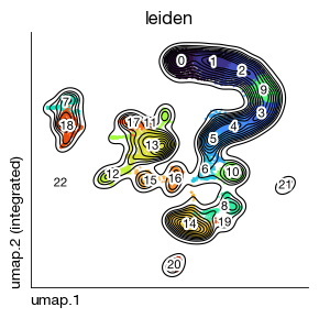
After loading the integrated experiment, we apply Leiden clustering on the pre-computed Harmony embedding to partition cells into discrete populations. The resolution parameter (0.8) balances the number of clusters — higher values yield finer subdivisions. The resulting clusters serve as the basis for downstream characterization and annotation.

[6]:

expm.rna.leiden(
    resolution = 0.8,
    restrict_to = None,
    random_state = 42,
    key_added = 'leiden',
    adjacency = None,
    directed = None,
    use_weights = True,
    n_iterations = 2,
    partition_type = None,
    neighbors_key = None,
    obsp = None,
    flavor = 'igraph'
)

[7]:

fig = expm.rna.plot_embedding(
    basis = 'umap', color = 'leiden',
    figsize = (3, 3), dpi = 100, legend_col = 2, legend = False,
    ptsize = 2, annotate_style = 'text', annotate_fontsize = 8, contour_plot = True
)

SC3 consensus clustering#

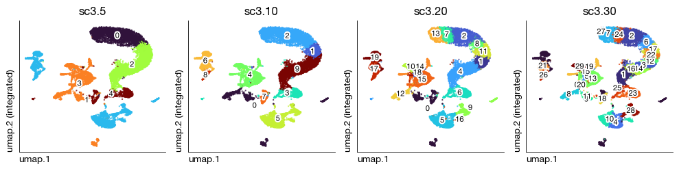
SC3 (Single-Cell Consensus Clustering) provides a complementary approach to Leiden clustering by combining multiple distance metrics and dimensionality reduction strategies through a consensus framework. It evaluates cluster stability across several values of k simultaneously, helping to identify the most robust partitions at different resolution scales. This is particularly useful for validating that the Leiden clusters represent stable biological populations rather than artifacts of the graph construction parameters.

[10]:

expm.rna.sc3(
    basis = 'harmony',
    key_added = 'sc3',
    n_clusters = [5, 10, 20, 30],
    d_range = None,
    n_runs = 5,
    n_facility = None,
    multiplier_facility = None,
    batch_size = None,
    random_state = 42
)

[i] multiplier_facility not set, using default value of 3
[i] number of facilities calculated as 90

[12]:

fig = expm.rna.plot_multiple_embedding(
    basis = 'umap', features = ['sc3.5', 'sc3.10', 'sc3.20', 'sc3.30'], ncols = 4,
    figsize = (10, 2.6), dpi = 100, legend_col = 2, legend = False,
    ptsize = 2, annotate_style = 'text', annotate_fontsize = 8
)

NMF-based metaprogram discovery#

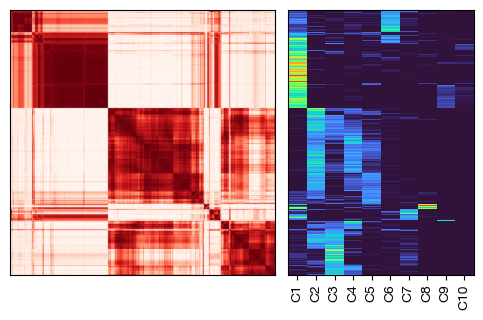
Non-negative matrix factorization (NMF) decomposes the gene expression matrix into two low-rank matrices: a gene-by-metaprogram matrix (W) and a metaprogram-by-cell matrix (H). Each metaprogram represents a co-expressed gene module, and cells are assigned membership scores for each module. Unlike clustering, NMF allows cells to belong to multiple programs simultaneously, capturing the continuous nature of cellular states. Consensus NMF (cNMF) runs the factorization multiple times with random initializations to identify stable, reproducible metaprograms across runs.

[13]:

# nmf requires linear normalized data
expm['rna'].layers['norm'] = em.np.expm1(expm['rna'].X)

[14]:

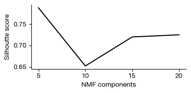
expm.rna.consensus_nmf(
    counts = 'counts', tpm = 'norm', ks = [5, 10, 15, 20],
    hvg = 'vst.all.hvg', ncpus = 50, key_added = 'cnmf', min_counts = 0
)

[15]:

fig = expm.rna.plot_cnmf_silhoutte(figsize = (4, 2))

[13]:

expm.rna.consensus_nmf_extract_k(k = 10)

[14]:

print(expm)

annotated data of size 13015 × 19651
integrated dataset of size 13015 × 19651
contains modalities: rna

 modality [rna]
    obs : sample <cat> <c/sample> batch <cat> <c/batch> group <cat> <c> modality <cat> <c/modality>
          taxa <cat> <c/taxa> barcode <o> <o> ubc <o> <o> n.umi <f64> <i> n.genes <i64> <i>
          n.mito <f64> <f> n.ribo <f64> <f> pct.mito <f64> <f> pct.ribo <f64> <f>
          filter <bool> <bool> score.doublet <f64> <f> score.doublet.se <f64> <f>
          is.doublet <bool> <bool> qc <bool> <bool/qc> leiden <cat> <c> sc3.5 <cat> <c>
          sc3.10 <cat> <c> sc3.20 <cat> <c> sc3.30 <cat> <c>
    var : chr <cat> <c/chromosome> start <i64> <i> end <i64> <i> strand <cat> <c/strand> id <o> <o>
          subtype <cat> <c/gsubtype> gene <cat> <o/gene> tlen <f64> <i/tlen> cdslen <i64> <i/cdslen>
          assembly <cat> <c> uid <o> <o/ugene> vst.hvg <bool> <bool/hvg> vst.all.means <f64> <f>
          vst.all.vars <f64> <f> vst.all.vars.norm <f64> <f> vst.all.hvg.rank <f32> <f>
          vst.all.hvg <bool> <bool>
 layers : counts <f32> <i/counts> norm <f32>
   obsm : cnmf.10 <df> <f/embedding/usage> harmony <arr:f32(35)> <f> knn <arr:i32(35)> <i>
          knn.d <arr:f32(35)> <f> pca <arr:f64(35)> <f/embedding/pca>
          umap <arr:f32(2)> <f/embedding>
   varm : cnmf.10 <arr:f64(10)> <f/weights> cnmf.coef.10 <arr:f64(10)> <f/usage-coef>
          pca <arr:f64(35)> <f/weights>
   obsp : connectivities <csr:f32> <f> distances <csr:f32> <f>
    uns : cnmf <cnmf> cnmf.args cnmf.density.10 <cnmf-density> cnmf.dist.10 <f/connectivity>
          cnmf.stats <cnmf-stats> commands <system> leiden <o> leiden.colors <o> neighbors <knn>
          pca <dict> sc3.10.colors sc3.20.colors sc3.30.colors sc3.5.colors slots <system> umap <o>

[*] composed of samples:
  distal   rna   mmu    batch b1      of size 6451 × 21689
  niche    rna   mmu    batch b2      of size 3656 × 21970
  normal   rna   mmu    batch b3      of size 4537 × 21917

[18]:

fig = expm.rna.plot_cnmf_distance_usages(
    k = 10, downsample = 0.1, method = 'complete', cmap = 'reds',
    cmap_annotations = 'turbo', annotations = 'cnmf.10', metrics = 'cosine',
    legend_cols = 1, figsize = (7, 3.3)
)

[23]:

fig = expm.rna.plot_cnmf_distance_modules(
    k = 10, downsample = 1, method = 'complete', cmap = 'reds',
    cmap_annotations = 'seismic', annotations = 'cnmf.coef.10', metrics = 'cosine',
    legend_cols = 1, figsize = (5, 3)
)

[27]:

expm.save()

[i] main dataset write to expm/scrna/integrated.h5mu
[i] saving individual samples. (pass `save_samples = False` to skip)

   ━━━━━━━━━━━━━━━━━━━━━━━━━━ modality [rna]           3 / 3     (00:01 < 00:00)

Manual annotation#

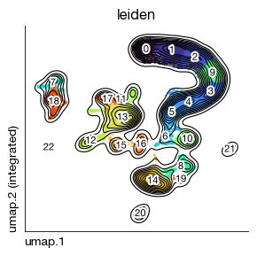
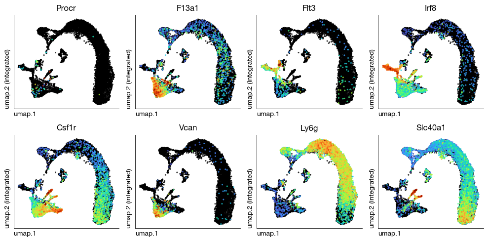
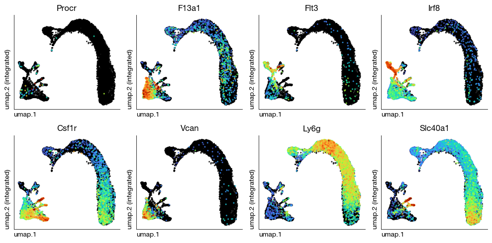
After unsupervised clustering and NMF decomposition, we assign biological cell type identities to each cluster based on the expression of canonical marker genes. This is an iterative process: we examine the distribution of known lineage markers across clusters, merge or split clusters as needed, and map them to biologically meaningful labels. We first visualize the Leiden clusters on the UMAP to identify major populations, then use known markers for hematopoietic progenitors (Procr), dendritic cell precursors (Flt3, Irf8), monocytes (Csf1r, Vcan), neutrophils (Ly6g), and macrophages (F13a1, Slc40a1) to guide the annotation.

[4]:

fig = expm.rna.plot_embedding(
    basis = 'umap', color = 'leiden',
    figsize = (3, 3), dpi = 100, legend_col = 2, legend = False,
    ptsize = 2, annotate_style = 'text', annotate_fontsize = 8, contour_plot = True
)

[15]:

expm.build_subset(
    subset_name = 'mono-neutro',
    slot = 'rna',
    keys = ['leiden'],
    values = [['0', '1', '2', '9', '3', '4', '5', '6', '10', '16', '15', '12', '13', '11', '17']]
)

[i] selected 10091 observations from 13015.

[16]:

expm = em.load_experiment('expm/scrna', load_samples = False, load_subset = 'mono-neutro')

[!] samples are not dumped in the experiment directory.

[19]:

expm.rna.knn(
    use_rep = 'harmony',
    n_comps = None,
    n_neighbors = 100,
    knn = True,
    method = "umap",
    transformer = None,
    metric = "euclidean",
    metric_kwds = {},
    random_state = 42,
    key_added = 'neighbors'
)

[20]:

expm.rna.umap(
    min_dist = 0.4,
    spread = 0.9,
    n_components = 2,
    maxiter = None,
    alpha = 1,
    gamma = 1,
    negative_sample_rate = 5,
    init_pos = "spectral",
    random_state = 42,
    a = None, b = None,
    key_added = 'umap',
    neighbors_key = "neighbors"
)

[21]:

expm.rna.leiden(
    resolution = 1,
    restrict_to = None,
    random_state = 42,
    key_added = 'leiden',
    adjacency = None,
    directed = None,
    use_weights = True,
    n_iterations = 2,
    partition_type = None,
    neighbors_key = None,
    obsp = None,
    flavor = 'igraph'
)

[22]:

print(expm)

annotated data of size 10091 × 19651
subset mono-neutro of size 10091 × 19651
contains modalities: rna

 modality [rna]
    obs : sample <cat> <c/sample> batch <cat> <c/batch> group <cat> <c> modality <cat> <c/modality>
          taxa <cat> <c/taxa> barcode <o> <o> ubc <o> <o> n.umi <f64> <i> n.genes <i64> <i>
          n.mito <f64> <f> n.ribo <f64> <f> pct.mito <f64> <f> pct.ribo <f64> <f>
          filter <bool> <bool> score.doublet <f64> <f> score.doublet.se <f64> <f>
          is.doublet <bool> <bool> qc <bool> <bool/qc> leiden <cat> <c> sc3.5 <cat> <c>
          sc3.10 <cat> <c> sc3.20 <cat> <c> sc3.30 <cat> <c>
    var : chr <cat> <c/chromosome> start <i64> <i> end <i64> <i> strand <cat> <c/strand> id <o> <o>
          subtype <cat> <c/gsubtype> gene <cat> <o/gene> tlen <f64> <i/tlen> cdslen <i64> <i/cdslen>
          assembly <cat> <c> uid <o> <o/ugene> vst.hvg <bool> <bool/hvg> vst.all.means <f64> <f>
          vst.all.vars <f64> <f> vst.all.vars.norm <f64> <f> vst.all.hvg.rank <f32> <f>
          vst.all.hvg <bool> <bool>
 layers : counts <f32> <i/counts> norm <f32> <f>
   obsm : cnmf.10 <df> <f/embedding/usage> harmony <arr:f32(35)> <f> knn <arr:i32(100)> <i/knni>
          knn.d <arr:f32(100)> <f/knnd> pca <arr:f64(35)> <f/embedding/pca>
          umap <arr:f32(2)> <f/embedding>
   varm : cnmf.10 <arr:f64(10)> <f/weights> cnmf.coef.10 <arr:f64(10)> <f/usage-coef>
          pca <arr:f64(35)> <f/weights>
   obsp : connectivities <csr:f32> <f/connectivity> distances <csr:f32> <f/distance>
    uns : cnmf <cnmf> cnmf.args <o> cnmf.density.10 <cnmf-density> cnmf.dist.10 <f/connectivity>
          cnmf.stats <cnmf-stats> commands <system> leiden <o> leiden.colors <o> neighbors <knn>
          pca <dict> sc3.10.colors <o> sc3.20.colors <o> sc3.30.colors <o> sc3.5.colors <o>
          slots <system> umap <o>

[*] samples not loaded from disk.

[23]:

fig = expm.rna.plot_embedding(
    basis = 'umap', color = 'leiden',
    figsize = (3, 3), dpi = 100, legend_col = 2, legend = False,
    ptsize = 2, annotate_style = 'text', annotate_fontsize = 8, contour_plot = True
)

[26]:

fig = expm.rna.plot_multiple_embedding(
    basis = 'umap', features = [
        'Procr', 'F13a1', 'Flt3', 'Irf8',
        'Csf1r', 'Vcan', 'Ly6g', 'Slc40a1'
    ], ncols = 4,
    sort = True, figsize = (10, 5), dpi = 100, legend = False,
    annotate_style = 'text', annotate_fontsize = 8, ptsize = 4
)

[32]:

expm.rna.exclude(
    annotation = 'leiden',
    remove = ['8', '15']
)

[i] keep 9754 observations from 9831.

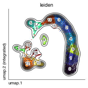
After reviewing the marker gene expression, we exclude clusters 8 and 15 as they likely represent contaminants or low-quality cells that do not match the monocyte-neutrophil lineage. The remaining cells are re-clustered with a higher resolution to resolve finer subpopulations within the myeloid compartment.

[33]:

expm.rna.knn(
    use_rep = 'harmony',
    n_comps = None,
    n_neighbors = 100,
    knn = True,
    method = "umap",
    transformer = None,
    metric = "euclidean",
    metric_kwds = {},
    random_state = 42,
    key_added = 'neighbors'
)

[34]:

expm.rna.umap(
    min_dist = 0.4,
    spread = 0.9,
    n_components = 2,
    maxiter = None,
    alpha = 1,
    gamma = 1,
    negative_sample_rate = 5,
    init_pos = "spectral",
    random_state = 42,
    a = None, b = None,
    key_added = 'umap',
    neighbors_key = "neighbors"
)

[35]:

fig = expm.rna.plot_multiple_embedding(
    basis = 'umap', features = [
        'Procr', 'F13a1', 'Flt3', 'Irf8',
        'Csf1r', 'Vcan', 'Ly6g', 'Slc40a1'
    ], ncols = 4,
    sort = True, figsize = (10, 5), dpi = 100, legend = False,
    annotate_style = 'text', annotate_fontsize = 8, ptsize = 4
)

[37]:

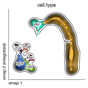
expm.rna.annotate(
    annotation = 'cell.type',
    cluster = 'leiden',
    mapping = {
        'Prog': [14],
        'DCp': [7],
        'MDP': [11, 12],
        'Mo': [10],
        'iMac': [16],
        'MM': [5, 6],
        'Neu': [13, 3, 2, 4, 9, 1, 0]
    }
)

cell.type
Neu     6706
MDP     1124
MM       707
Mo       479
DCp      282
Prog     235
iMac     221
Name: count, dtype: int64

[38]:

fig = expm.rna.plot_embedding(
    basis = 'umap', color = 'cell.type',
    figsize = (3, 3), dpi = 100, legend_col = 2, legend = False,
    ptsize = 2, annotate_style = 'text', annotate_fontsize = 8, contour_plot = True
)

[39]:

expm.rna.markers(
    groupby = 'cell.type',
    mask_var = None,
    groups = 'all',
    reference = 'rest',
    n_genes = None, rankby_abs = False, pts = True,
    key_added = 'markers',
    method = 't-test',
    corr_method = 'benjamini-hochberg',
    tie_correct = False,
    gene_symbol = 'gene',
    layer = 'X'
)

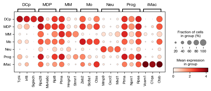
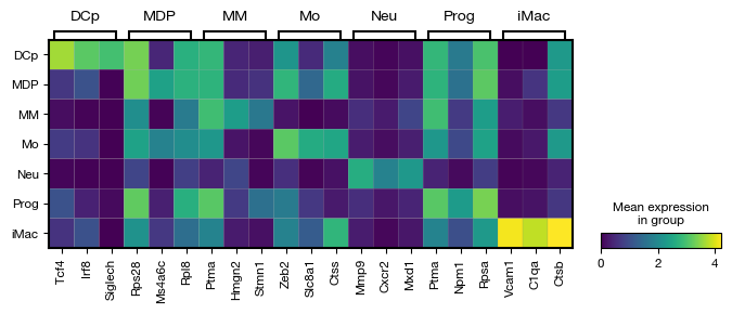
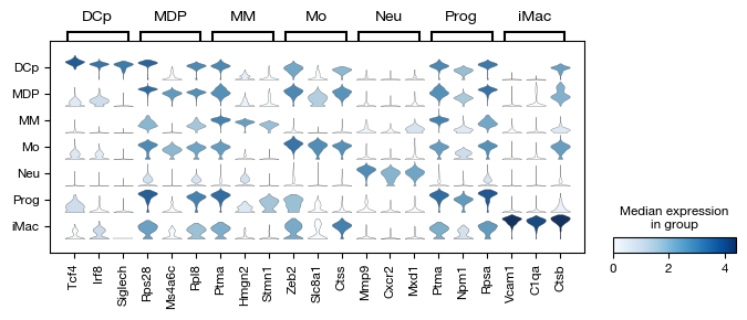
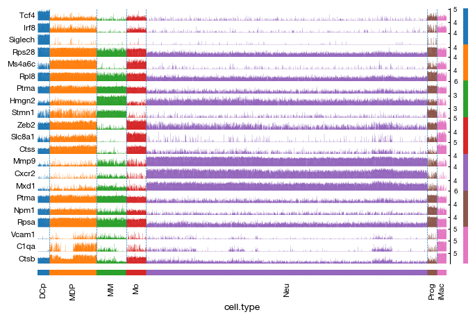
After assigning cell type labels, we identify differentially expressed marker genes for each annotated population using a t-test. The marker analysis compares each cell type against all others (reference='rest') to find genes that are specifically upregulated in each population. The results are corrected for multiple testing using the Benjamini-Hochberg procedure and include the percentage of cells expressing each gene in both the target and reference groups for interpretability.

[45]:

fig = expm.rna.plot_markers(
    n_genes = 3,
    groupby = 'cell.type',
    min_logfoldchange = 1,
    max_logfoldchange = None,
    max_p_adjust = 0.05,
    min_pct = 0.25,
    max_pct_reference = 0.75,
    key = 'markers',
    gene_symbols = 'gene',
    figsize = (8, 2.5),
    dpi = 100,
    plot_type = 'dotplot'
)

[46]:

fig = expm.rna.plot_markers(
    n_genes = 3,
    groupby = 'cell.type',
    min_logfoldchange = 1,
    max_logfoldchange = None,
    max_p_adjust = 0.05,
    min_pct = 0.25,
    max_pct_reference = 0.75,
    key = 'markers',
    gene_symbols = 'gene',
    figsize = (8, 2.5),
    dpi = 100,
    plot_type = 'matrixplot'
)

[47]:

fig = expm.rna.plot_markers(
    n_genes = 3,
    groupby = 'cell.type',
    min_logfoldchange = 1,
    max_logfoldchange = None,
    max_p_adjust = 0.05,
    min_pct = 0.25,
    max_pct_reference = 0.75,
    key = 'markers',
    gene_symbols = 'gene',
    figsize = (8, 2.5),
    dpi = 100,
    plot_type = 'stacked_violin'
)

[50]:

fig = expm.rna.plot_markers(
    n_genes = 3,
    groupby = 'cell.type',
    min_logfoldchange = 1,
    max_logfoldchange = None,
    max_p_adjust = 0.05,
    min_pct = 0.25,
    max_pct_reference = 0.75,
    key = 'markers',
    gene_symbols = 'gene',
    figsize = (8, 5),
    dpi = 100,
    plot_type = 'tracksplot'
)

Proportions of subtypes#

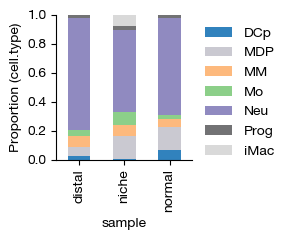
Finally, we examine the compositional differences across experimental groups by calculating the proportion of each cell type within each sample. This reveals how the cellular landscape shifts between conditions — for instance, whether certain myeloid populations are enriched or depleted in the distal bone marrow niche compared to normal marrow.

[51]:

fig = expm.rna.plot_proportion(
    major = 'sample', minor = 'cell.type', plot = 'bar', cmap = 'category20c',
    normalize = 'index', figsize = (3, 2.5), stacked = True, legend = True
)

[53]:

expm.rna.proportion(
    major = 'sample', minor = 'cell.type',
    normalize = 'index'
)['integrated']

[53]:

cell.type	DCp	MDP	MM	Mo	Neu	Prog	iMac
sample
distal	0.023297	0.062052	0.080421	0.035842	0.774194	0.023970	0.000224
niche	0.001878	0.160345	0.079985	0.088246	0.563275	0.024784	0.081487
normal	0.065855	0.159878	0.051389	0.031976	0.666159	0.023601	0.001142

[55]:

print(expm)

annotated data of size 9754 × 19651
subset mono-neutro of size 9754 × 19651
contains modalities: rna

 modality [rna]
    obs : sample <cat> <c/sample> batch <cat> <c/batch> group <cat> <c> modality <cat> <c/modality>
          taxa <cat> <c/taxa> barcode <o> <o> ubc <o> <o> n.umi <f64> <i> n.genes <i64> <i>
          n.mito <f64> <f> n.ribo <f64> <f> pct.mito <f64> <f> pct.ribo <f64> <f>
          filter <bool> <bool> score.doublet <f64> <f> score.doublet.se <f64> <f>
          is.doublet <bool> <bool> qc <bool> <bool/qc> leiden <cat> <c> sc3.5 <cat> <c>
          sc3.10 <cat> <c> sc3.20 <cat> <c> sc3.30 <cat> <c> cell.type <cat> <c>
    var : chr <cat> <c/chromosome> start <i64> <i> end <i64> <i> strand <cat> <c/strand> id <o> <o>
          subtype <cat> <c/gsubtype> gene <cat> <o/gene> tlen <f64> <i/tlen> cdslen <i64> <i/cdslen>
          assembly <cat> <c> uid <o> <o/ugene> vst.hvg <bool> <bool/hvg> vst.all.means <f64> <f>
          vst.all.vars <f64> <f> vst.all.vars.norm <f64> <f> vst.all.hvg.rank <f32> <f>
          vst.all.hvg <bool> <bool>
 layers : counts <f32> <i/counts> norm <f32> <f>
   obsm : cnmf.10 <df> <f/embedding/usage> harmony <arr:f32(35)> <f> knn <arr:i32(100)> <i/knni>
          knn.d <arr:f32(100)> <f/knnd> pca <arr:f64(35)> <f/embedding/pca>
          umap <arr:f32(2)> <f/embedding>
   varm : cnmf.10 <arr:f64(10)> <f/weights> cnmf.coef.10 <arr:f64(10)> <f/usage-coef>
          pca <arr:f64(35)> <f/weights>
   obsp : connectivities <csr:f32> <f/connectivity> distances <csr:f32> <f/distance>
    uns : cnmf <cnmf> cnmf.args <o> cnmf.density.10 <cnmf-density> cnmf.dist.10 <f/connectivity>
          cnmf.stats <cnmf-stats> commands <system> leiden <o> leiden.colors <o> neighbors <knn>
          pca <dict> sc3.10.colors <o> sc3.20.colors <o> sc3.30.colors <o> sc3.5.colors <o>
          slots <system> umap <o> cell.type.colors markers <markers> cell.type_colors

[*] samples not loaded from disk.

[54]:

expm.save()

[i] main dataset write to expm/scrna/subsets/mono-neutro.h5mu