Differential Accessibility Analysis#
Once we have a peak-by-sample count matrix, we can identify chromatin regions that show statistically significant differences in accessibility between experimental conditions. Furthermore, we can discover conserved transcription factor binding motifs within these differentially accessible regions, providing mechanistic insights into the regulatory programs underlying phenotypic differences.
Analysis workflow:
Annotate peaks to nearby genes
Identify differentially accessible peaks (DESeq2)
Visualize differential peaks at key loci
Extract peak sequences from the reference genome
Match sequences against known motif databases (JASPAR)
Test motifs for enrichment in differential vs. background peaks
Visualize sequence logos and transcription factor footprints
Compute ChromVAR motif variability scores across samples
[1]:
%load_ext autoreload
%autoreload 2
[2]:
import exprmat as em

em.setwd('../../../data')
ver = em.version()
[i] exprmat 0.2.66 / exprmat-db 0.2.66
[i] os: posix (linux)  platform version: 6.8.0-90-generic
[i] loaded configuration from /home/data/yangz/.exprmatrc
[i] current working directory: /home/data/yangz/packages/exprmat/data
[i] current database directory: /home/data/yangz/packages/database (0.2.66)
[i] resident memory: 778.63 MiB
[i] virtual memory: 5.95 GiB
[3]:
expm = em.load_experiment('expm/bk-atac')
━━━━━━━━━━━━━━━━━━━━━━━━━━ loading samples 2 / 2 (00:04 < 00:00)
[!] integrated mudata object is not generated.
[4]:
expm.atac['bulk-atac'].obs
[4]:
| n.fragments | pct.dup | pct.mito | location | sample | batch | group | modality | taxa | tsse | |
|---|---|---|---|---|---|---|---|---|---|---|
| bulk-atac:c1 | 25596750 | 0.000264 | 0.0 | atac/control-1.bam | c1 | b-1 | control | atac-bulk | hsa/grch38 | 7.181466 |
| bulk-atac:c2 | 29933508 | 0.000356 | 0.0 | atac/control-2.bam | c2 | b-1 | control | atac-bulk | hsa/grch38 | 4.210467 |
| bulk-atac:c3 | 26024477 | 0.000272 | 0.0 | atac/control-3.bam | c3 | b-1 | control | atac-bulk | hsa/grch38 | 7.388964 |
| bulk-atac:e1 | 24406481 | 0.000328 | 0.0 | atac/hp-1.bam | e1 | b-1 | expm | atac-bulk | hsa/grch38 | 9.118949 |
| bulk-atac:e2 | 26010889 | 0.000294 | 0.0 | atac/hp-2.bam | e2 | b-1 | expm | atac-bulk | hsa/grch38 | 7.051591 |
| bulk-atac:e3 | 23710917 | 0.000301 | 0.0 | atac/hp-3.bam | e3 | b-1 | expm | atac-bulk | hsa/grch38 | 8.239926 |
[5]:
print(expm)
[!] dataset not integrated.
[*] composed of samples:
  bulk-atac   atac      hsa    batch autogen   of size 6 × 0
  bulk-atac   atac-peak hsa    batch autogen   of size 6 × 48519
[6]:
expm.atac.view('bulk-atac')
annotated data of size 6 × 0
    obs : n.fragments <ui64> <i> pct.dup <f64> <f> pct.mito <f64> <f> location <o> <o/location>
          sample <o> <c/sample> batch <cat> <c/batch> group <cat> <c> modality <cat> <c/modality>
          taxa <cat> <c/taxa> tsse <f64> <f/tsse>
   obsm : paired <csr:ui32(3088286401)> <fragments>
    uns : assembly <assembly> assembly.size <asm-size> frag.sizes <frag-size>
          pct.tss.overlap <tss-overlap> peaks.group <dict/peaks/grouped-peaks>
          peaks.merged <dict/peaks/merged-peaks> tss.profile <tss-profile> tsse <overall-tsse>
[7]:
expm.atac_peak.view('bulk-atac')
annotated data of size 6 × 48519
    obs : n.fragments <ui64> <i> pct.dup <f64> <f> pct.mito <f64> <f> location <o> <o/location>
          sample <o> <c/sample> batch <cat> <c/batch> group <cat> <c> modality <cat> <c/modality>
          taxa <cat> <c/taxa> tsse <f64> <f/tsse>
    var : expm <bool> <bool> control <bool> <bool> chr <cat> <c/chromosome> start <i64> <i>
          end <i64> <i> strand <cat> <o/strand> summit <i64> <i>
    uns : assembly <assembly> assembly.size <asm-size>
[9]:
expm.atac_peak.list_available_tools('bulk-atac', light = True)
[9]:
[{'tool': 'annotate_peak', 'kind': 'computation'},
 {'tool': 'expression_linkage', 'kind': 'computation'},
 {'tool': 'retrieve_sequence', 'kind': 'computation'}]
Annotating Peaks to Genes#
ATAC-seq peaks represent open chromatin regions, but they don’t come with gene names. A common and simple annotation strategy is the nearest TSS (transcription start site) method:
For each peak, find the nearest annotated TSS in the reference genome
Record the distance (in bp) from the peak center/summit to the TSS
Classify peaks by genomic context:
Promoter: Within ±2 kb of a TSS
Proximal: 2-10 kb from a TSS
Distal intergenic: >10 kb from any TSS (potential enhancers)
Intronic / Exonic: Overlapping gene bodies
The annotation adds columns to .var including:
type: Genomic region classificationtss.nearest: Distance to the nearest TSSugene: Ensembl gene IDgene: Gene symboltss.dist: Signed distance to TSS (negative = upstream)
Caveat: The nearest-TSS approach is simplistic. Enhancers can regulate genes hundreds of kb away, and the nearest gene is not always the regulatory target. More sophisticated methods (e.g., correlation-based linking, Hi-C) exist but are beyond this tutorial.
[10]:
expm.atac_peak.annotate_peak(run_on_samples = ['bulk-atac'])
[11]:
expm.atac_peak.view('bulk-atac')
annotated data of size 6 × 48519
    obs : n.fragments <ui64> <i> pct.dup <f64> <f> pct.mito <f64> <f> location <o> <o/location>
          sample <o> <c/sample> batch <cat> <c/batch> group <cat> <c> modality <cat> <c/modality>
          taxa <cat> <c/taxa> tsse <f64> <f/tsse>
    var : expm <bool> <bool> control <bool> <bool> chr <cat> <c/chromosome> start <i64> <i>
          end <i64> <i> strand <cat> <o/strand> summit <i64> <i> type <o> <c/genomic-annot>
          tss.nearest <o> <o> ugene <o> <o/ugene> gene <o> <o/gene> tss.dist <f64> <i>
    uns : assembly <assembly> assembly.size <asm-size>
[13]:
expm.atac_peak['bulk-atac'].var[['type', 'tss.nearest', 'ugene', 'gene', 'tss.dist']]
[13]:
| type | tss.nearest | ugene | gene | tss.dist | |
|---|---|---|---|---|---|
| peak:grch38:chr1:9853-10354 | promoter | ENSG00000290825 | rna:hsa:g1 | DDX11L16 | -1016.0 |
| peak:grch38:chr1:15983-16484 | promoter | ENSG00000310526 | rna:hsa:g2 | WASH7P | -865.0 |
| peak:grch38:chr1:181228-181729 | promoter | ENSG00000308415 | rna:hsa:g18 | DDX11L2 | 147.0 |
| peak:grch38:chr1:180549-181050 | promoter | ENSG00000308415 | rna:hsa:g18 | DDX11L2 | -130.0 |
| peak:grch38:chr1:191240-191741 | first-intron | ENSG00000310527 | rna:hsa:g19 | WASH9P | 1386.0 |
| ... | ... | ... | ... | ... | ... |
| peak:grch38:chrY:56706793-56707294 | intergenic | ENSG00000235857 | rna:hsa:g78922 | CTBP2P1 | -148199.0 |
| peak:grch38:chrY:56727895-56728396 | intergenic | ENSG00000235857 | rna:hsa:g78922 | CTBP2P1 | -127097.0 |
| peak:grch38:chrY:56734538-56735039 | intergenic | ENSG00000235857 | rna:hsa:g78922 | CTBP2P1 | -120454.0 |
| peak:grch38:chrY:56742463-56742964 | intergenic | ENSG00000235857 | rna:hsa:g78922 | CTBP2P1 | -112529.0 |
| peak:grch38:chrY:56763268-56763769 | intergenic | ENSG00000235857 | rna:hsa:g78922 | CTBP2P1 | -91724.0 |
48519 rows × 5 columns
Differential Accessibility Analysis with DESeq2#
To identify peaks that are significantly more or less accessible between conditions, we use the DESeq2 method — originally developed for bulk RNA-seq differential expression analysis, but widely adapted for ATAC-seq differential peak analysis.
Why DESeq2 for ATAC-seq peaks?
ATAC-seq peak counts are count data (integer values), similar to RNA-seq read counts
Peaks exhibit overdispersion (variance > mean), which DESeq2 handles via negative binomial modeling
DESeq2 uses empirical Bayes shrinkage to stabilize dispersion estimates for low-count peaks
The model accounts for library size differences via size factor normalization
Statistical model: $ \text{Count} \sim `:nbsphinx-math:text{NB}`(\mu, \alpha) $ $ \log`(:nbsphinx-math:mu`) = \beta_0 + \beta_1 \cdot `:nbsphinx-math:text{condition}` $
Where:
\(\mu\) is the mean count (adjusted for library size)
\(\alpha\) is the dispersion parameter
\(\beta_1\) is the log2 fold change between conditions
Parameters:
formula='~ group': Model accessibility as a function of biological groupvariable='group': The variable of interest for contrastexperiment='expm',control='control': Defines the comparison direction (expm vs control)
[15]:
expm.atac_peak.markers_deseq(
    run_on_samples = ['bulk-atac'], counts = 'X',
    metadata = ['sample', 'group'], formula = '~ group',
    variable = 'group', experiment = 'expm', control = 'control',
)
[i] fitting size factors ...
[i] using None as control genes, passed at deseq_dataset initialization
[i]   done in 0.01 seconds.
[i] fitting dispersions...
[i]   done in 7.14 seconds.
[i] fitting dispersion trend curve ...
[i]   done in 0.83 seconds.
[i] fitting map dispersions ...
[i]   done in 5.02 seconds.
[i] fitting log fold changes ...
[i]   done in 9.43 seconds.
[i] calculating cook's distance ...
[i]   done in 0.02 seconds.
[i] replacing 0 outlier genes.
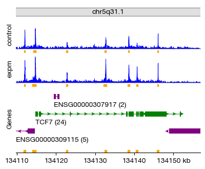
For example, we can filter for differentially accessible peaks near the TCF7 locus — a key transcription factor in T-cell development and function. The results show peaks annotated to TCF7 with their mean accessibility, log2 fold change (lfc), and statistical significance (q-value).
[ ]:
upreg = expm.atac_peak.get_markers(
    run_on_samples = ['bulk-atac'],
    de_slot = 'markers', max_q = 1,
    min_lfc = 0.1, max_lfc = 10000
)['bulk-atac-peaks'][
    ['mean', 'lfc', 'lfc.se', 'names', 'gene', 'q']
].sort_values('lfc')

upreg.loc[upreg['gene'] == 'TCF7', :]
[i] fetched diff `expm` over `control` (14047 genes)
| mean | lfc | lfc.se | names | gene | q | |
|---|---|---|---|---|---|---|
| 37300 | 29.540347 | 0.156705 | 0.336371 | peak:grch38:chr5:134113861-134114362 | TCF7 | 0.999857 |
| 37302 | 60.085868 | 0.259853 | 0.241759 | peak:grch38:chr5:134132392-134132893 | TCF7 | 0.999857 |
| 37304 | 30.137926 | 0.752380 | 0.323924 | peak:grch38:chr5:134140398-134140899 | TCF7 | 0.999857 |
[20]:
figs = expm.atac.plot_peaks(
    run_on_samples = ['bulk-atac'],
    group_key = 'group', peaks_key = 'peaks.group',
    # either specifying a gene name for convenience
    gene = 'TCF7', upstream = 5000, downstream = 5000,
    # or specify chromosome coordinates manually
    chr = None, xf = None, xt = None,
    figsize = (4, 3.2), dpi = 100,
    gene_track_height = 0.45, chrom_track_height = 0.10,
    peak_annotation_height = 0.1,
    min_frag_length = None, max_frag_length = 180,
    plot_consensus_peak = 'peaks.merged',
    title = None, showgn = True,

    do_tight_layout = False
)
Extracting Peak Sequences#
To analyze motif enrichment within differentially accessible peaks, we first need to extract the underlying DNA sequences from the reference genome. The run_atacp_retrieve_sequence() function:
Takes each peak interval (chromosome, start, end)
Extracts the corresponding nucleotide sequence from the reference genome
Optionally extends the sequence to a fixed length (
seqlen=200bp) centered on the peak summitStores the sequences for downstream motif analysis
The extracted sequences are stored in the .var DataFrame, where each row contains the genomic coordinates and the retrieved sequence.
[17]:
expm.atac_peak.retrieve_sequence(
    run_on_samples = ['bulk-atac'],
    seqlen = 200
)
━━━━━━━━━━━━━━━━━━━━━━━━━━ fetching chromosome 24 / 24 (00:18 < 00:00)
[18]:
expm.atac_peak['bulk-atac'].var[['strand.pos']]
[18]:
| strand.pos | |
|---|---|
| peak:grch38:chr1:9853-10354 | ACCCTAACCCTAACCCTAACCCTAACCCTAACCCTAACCCTAACCC... |
| peak:grch38:chr1:15983-16484 | CCTGAGCGCGGGCATCCTGTGTGCAGATACTCCCTGCTTCCTCTCT... |
| peak:grch38:chr1:181228-181729 | GGCGCAGAGACACATGCTAGCGCGCCCAGGGGAGGAGGCGTGGCGC... |
| peak:grch38:chr1:180549-181050 | CCTAACCCTAACCCTACCCTAACCCAACCCTAACCCAACCCTAACT... |
| peak:grch38:chr1:191240-191741 | TGACTGTCATCCCCTCCAGTCTCTGCACACTCCCAGCTGCAGCAGA... |
| ... | ... |
| peak:grch38:chrY:56706793-56707294 | GGAATGGAGTGCAGTGCAATGGAATGGAATGGAATGGAATGCAATG... |
| peak:grch38:chrY:56727895-56728396 | ATGGAATGGAATCGAATGCAATGGAATGCTATGGAATGGAATGGAA... |
| peak:grch38:chrY:56734538-56735039 | AAAGGAATCGAATGGAAGGGAATGAAATTGAATCAACACGAATGGA... |
| peak:grch38:chrY:56742463-56742964 | AATGTAATGGAATGGAGTGCAGTGCAATGGAATGGAATGGAATGGA... |
| peak:grch38:chrY:56763268-56763769 | GAATAGAATGGAACGAAATTTCACGGAATGGAATCAAACTGAATGG... |
48519 rows × 1 columns
[19]:
expm.atac_peak.view('bulk-atac')
annotated data of size 6 × 48519
    obs : n.fragments <ui64> <i> pct.dup <f64> <f> pct.mito <f64> <f> location <o> <o/location>
          sample <o> <c/sample> batch <cat> <c/batch> group <cat> <c> modality <cat> <c/modality>
          taxa <cat> <c/taxa> tsse <f64> <f/tsse>
    var : expm <bool> <bool> control <bool> <bool> chr <cat> <c/chromosome> start <i64> <i>
          end <i64> <i> strand <cat> <o/strand> summit <i64> <i> type <o> <c/genomic-annot>
          tss.nearest <o> <o> ugene <o> <o/ugene> gene <o> <o/gene> tss.dist <f64> <i>
          strand.pos <o> <o/sequence> strand.neg <o> <o/sequence>
    uns : assembly <assembly> assembly.size <asm-size> markers
[20]:
expm.atac_peak.list_available_tools('bulk-atac', True)
[20]:
[{'tool': 'annotate_peak', 'kind': 'computation'},
 {'tool': 'expression_linkage', 'kind': 'computation'},
 {'tool': 'motif_match', 'kind': 'computation'},
 {'tool': 'retrieve_sequence', 'kind': 'computation'}]
Next, we scan the extracted peak sequences against known transcription factor motifs from the JASPAR database. The run_atacp_motif_match() function:
Uses curated position weight matrices (PWMs) from the JASPAR database (a comprehensive collection of eukaryotic transcription factor binding profiles)
Scans each peak sequence for motif occurrences using a sliding window approach
Scores each position using a log-likelihood ratio (motif score vs. background)
Calls a motif match when the score exceeds a threshold (default: p < 1e-5)
Parameters:
subset='jaspar': Use only JASPAR-annotated motifs (high-quality, curated)length=200: The sequence window length to scanthreshold=0.00001: Stringent p-value threshold for motif matching
The results store the position and score of each motif match within each peak.
[21]:
expm.atac_peak.motif_match(
    run_on_samples = ['bulk-atac'],
    motif_matches = 'motifs',
    subset = 'jaspar',
    length = 200,
    threshold = 0.00001
)
━━━━━━━━━━━━━━━━━━━━━━━━━━ generating pssm 10249 / 10249 (00:00 < 00:00)
[i] matching motifs for foreground ...
━━━━━━━━━━━━━━━━━━━━━━━━━━ foreground matching 1936 / 1936 (02:49 < 00:00)
[22]:
expm.atac_peak.list_available_tools('bulk-atac', True)
[22]:
[{'tool': 'annotate_peak', 'kind': 'computation'},
 {'tool': 'chromvar', 'kind': 'computation'},
 {'tool': 'expression_linkage', 'kind': 'computation'},
 {'tool': 'footprint', 'kind': 'computation'},
 {'tool': 'motif_enrichment', 'kind': 'computation'},
 {'tool': 'motif_match', 'kind': 'computation'},
 {'tool': 'retrieve_sequence', 'kind': 'computation'}]
After identifying motif occurrences, we perform a statistical enrichment test to determine which motifs are significantly overrepresented in differentially accessible peaks compared to a background set.
Enrichment method:
Foreground: The set of differentially accessible peaks (e.g., upregulated in experimental condition)
Background: A matched set of non-differential peaks (by default, randomly sampled from all peaks)
Contingency table: Count motif occurrences in foreground vs. background
Statistical test: Chi-squared test (or Fisher’s exact test for small counts) on the 2×2 contingency table
Parameters:
background='background': Use the background model to sample matched null peaksn=5000: Sample 5,000 background peaks for comparisonrandom_seed=42: Reproducible random sampling
[23]:
expm.atac_peak.motif_enrichment(
    run_on_samples = ['bulk-atac'],
    background = 'background',
    n = 5000,
    length = 200,
    random_seed = 42,
    threshold = 0.00001,
    motif_matches = 'motifs',
    key_added = 'motifs.enrich',
    subset = 'jaspar'
)
━━━━━━━━━━━━━━━━━━━━━━━━━━ generating pssm 10249 / 10249 (00:00 < 00:00)
[i] generating background regions ...
[i] fetching chromosomes, round 1 ...
[i] fetching chromosomes, round 2 ...
[i] fetching chromosomes, round 3 ...
[i] fetching chromosomes, round 4 ...
[i] fetching chromosomes, round 5 ...
[i] fetching chromosomes, round 6 ...
[i] fetching chromosomes, round 7 ...
[i] fetching chromosomes, round 8 ...
[i] fetching chromosomes, round 9 ...
[i] fetching chromosomes, round 10 ...
[i] fetching chromosomes, round 11 ...
[i] matching motifs for background ...
━━━━━━━━━━━━━━━━━━━━━━━━━━ background matching 1936 / 1936 (00:05 < 00:00)
We can examine the results table, sorted by statistical significance (chi-squared statistic, descending). This reveals which transcription factor motifs are most strongly enriched in the differential peaks, suggesting which regulatory programs may be driving the chromatin response.
[24]:
m = expm.atac_peak['bulk-atac'].uns['motifs.enrich'].copy()
m.loc[~m['chisq'].isna(), :].sort_values('chisq', ascending = False)
[24]:
| motif | fg.hit | fg | gc | bg.hit | bg | fg.ratio | bg.ratio | fc | chisq | p | log10.p | |
|---|---|---|---|---|---|---|---|---|---|---|---|---|
| 1255 | motif:18810 | 934 | 48519 | 0.560541 | 529 | 5000 | 0.019250 | 0.1058 | 0.181949 | 1.277047e+03 | 0.000000 | inf |
| 731 | motif:18013 | 7062 | 48519 | 0.580299 | 31 | 5000 | 0.145551 | 0.0062 | 23.476004 | 7.656322e+02 | 0.000000 | inf |
| 1150 | motif:18349 | 229 | 48519 | 0.520852 | 194 | 5000 | 0.004720 | 0.0388 | 0.121644 | 6.714164e+02 | 0.000000 | inf |
| 1175 | motif:18478 | 200 | 48519 | 0.507400 | 144 | 5000 | 0.004122 | 0.0288 | 0.143128 | 4.322554e+02 | 0.000000 | inf |
| 734 | motif:19009 | 4501 | 48519 | 0.594672 | 42 | 5000 | 0.092768 | 0.0084 | 11.043784 | 4.153527e+02 | 0.000000 | inf |
| ... | ... | ... | ... | ... | ... | ... | ... | ... | ... | ... | ... | ... |
| 1501 | motif:36464 | 78 | 48519 | 0.457179 | 8 | 5000 | 0.001608 | 0.0016 | 1.004761 | 1.639540e-04 | 0.989784 | 0.004460 |
| 536 | motif:18443 | 116 | 48519 | 0.634914 | 12 | 5000 | 0.002391 | 0.0024 | 0.996173 | 1.602428e-04 | 0.989900 | 0.004409 |
| 554 | motif:18530 | 39 | 48519 | 0.483974 | 4 | 5000 | 0.000804 | 0.0008 | 1.004761 | 8.191109e-05 | 0.992779 | 0.003147 |
| 388 | motif:18578 | 184 | 48519 | 0.489103 | 19 | 5000 | 0.003792 | 0.0038 | 0.997981 | 7.059359e-05 | 0.993296 | 0.002921 |
| 665 | motif:35629 | 165 | 48519 | 0.440455 | 17 | 5000 | 0.003401 | 0.0034 | 1.000215 | 7.119881e-07 | 0.999327 | 0.000292 |
1532 rows × 12 columns
[26]:
expm.atac_peak.view('bulk-atac')
annotated data of size 6 × 48519
    obs : n.fragments <ui64> <i> pct.dup <f64> <f> pct.mito <f64> <f> location <o> <o/location>
          sample <o> <c/sample> batch <cat> <c/batch> group <cat> <c> modality <cat> <c/modality>
          taxa <cat> <c/taxa> tsse <f64> <f/tsse>
    var : expm <bool> <bool> control <bool> <bool> chr <cat> <c/chromosome> start <i64> <i>
          end <i64> <i> strand <cat> <o/strand> summit <i64> <i> type <o> <c/genomic-annot>
          tss.nearest <o> <o> ugene <o> <o/ugene> gene <o> <o/gene> tss.dist <f64> <i>
          strand.pos <o> <o/sequence> strand.neg <o> <o/sequence>
   varm : motifs <csc:ui8(1936)> <f/motif-matches> motifs.locs <csc:i32(1936)>
    uns : assembly <assembly> assembly.size <asm-size> markers motifs.names motifs.seqlen
          background <motif-background> motifs.enrich <motif-enrich>
Motif Visualization#
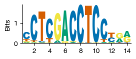
The motif IDs in the enrichment table (e.g., motif:18810) are internal codes referencing the exprmat motif database. We can visualize a motif’s sequence logo — a graphical representation of its position weight matrix:
The x-axis shows the position within the motif (in bp)
The y-axis shows the information content (bits), ranging from 0 (completely random) to 2 (perfectly conserved)
Each nucleotide (A, C, G, T) is stacked at each position, with its height proportional to its frequency
Taller stacks indicate more conserved positions
Sequence logos are generated using the plot_sequence_logo() function.
[34]:
from exprmat.data.cre import plot_sequence_logo, search_transcription_factor

mot = plot_sequence_logo('motif:18810')
We can also query the database for transcription factor - motif associations. For example, to find which JASPAR motifs are known to be bound by TCF7 (TCF1), a T-cell-specific transcription factor. This helps interpret which enriched motifs correspond to biologically relevant regulators.
[35]:
search_transcription_factor('hsa', 'TCF7', 'jaspar')
[35]:
[('mc:311', 'motif:18190'),
 ('mc:311', 'motif:18688'),
 ('mc:311', 'motif:19071'),
 ('mc:4295', 'motif:18389'),
 ('mc:119', 'motif:18944'),
 ('mc:119', 'motif:18945'),
 ('mc:119', 'motif:18948'),
 ('mc:119', 'motif:18952'),
 ('mc:119', 'motif:18953'),
 ('mc:9071', 'motif:18390')]
Transcription Factor Footprint Analysis#
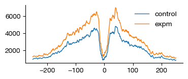
When a transcription factor binds to its cognate motif, it protects the underlying DNA from Tn5 transposition. This creates a footprint — a local dip in the Tn5 cut frequency centered on the binding site, flanked by increased accessibility (the “open” chromatin shoulders).
The run_atacp_footprint() function:
Identifies all motif occurrences in the genome
For each occurrence, aggregates the Tn5 cut frequency ±250 bp around the motif center
Normalizes by the average cut frequency in flanking regions
Produces a meta-profile showing the average footprint pattern
Interpreting footprints:
A clear dip at the motif center indicates active TF binding
Flanking peaks correspond to accessible regions around the protected binding site
Differences between conditions (e.g., control vs. experimental) reveal condition-specific TF binding
Here we compute the footprint for motif motif:18944 (TCF7 binding motif) and visualize the resulting profile.
[28]:
expm.atac_peak.footprint(
    run_on_samples = ['bulk-atac'],
    adata_atac = expm.atac['bulk-atac'],
    motif = 'motif:18944',
    motif_matches = 'motifs',
    groupby = 'group',
    key_added = 'footprint.tcf7-1'
)
   ━━━━━━━━━━━━━━━━━━━━━━━━━━ summarizing peaks     1075 / 1075  (02:30 < 00:00)
   ━━━━━━━━━━━━━━━━━━━━━━━━━━ summarizing peaks     1075 / 1075  (02:00 < 00:00)
[30]:
from exprmat.plotting.utils import line

fig = line(
    x = [x - 250 for x in range(501)],
    y = expm.atac_peak['bulk-atac'].uns['footprint.tcf7-1'],
    figsize = (4, 1.5),
)
[31]:
expm.atac_peak.view('bulk-atac')
annotated data of size 6 × 48519
    obs : n.fragments <ui64> <i> pct.dup <f64> <f> pct.mito <f64> <f> location <o> <o/location>
          sample <o> <c/sample> batch <cat> <c/batch> group <cat> <c> modality <cat> <c/modality>
          taxa <cat> <c/taxa> tsse <f64> <f/tsse>
    var : expm <bool> <bool> control <bool> <bool> chr <cat> <c/chromosome> start <i64> <i>
          end <i64> <i> strand <cat> <o/strand> summit <i64> <i> type <o> <c/genomic-annot>
          tss.nearest <o> <o> ugene <o> <o/ugene> gene <o> <o/gene> tss.dist <f64> <i>
          strand.pos <o> <o/sequence> strand.neg <o> <o/sequence>
   varm : motifs <csc:ui8(1936)> <f/motif-matches> motifs.locs <csc:i32(1936)>
    uns : assembly <assembly> assembly.size <asm-size> markers motifs.names motifs.seqlen
          background <motif-background> motifs.enrich <motif-enrich> footprint.tcf7-1 <footprint>
[35]:
expm.atac_peak.list_available_tools('bulk-atac', True)
[35]:
[{'tool': 'annotate_peak', 'kind': 'computation'},
 {'tool': 'chromvar', 'kind': 'computation'},
 {'tool': 'expression_linkage', 'kind': 'computation'},
 {'tool': 'footprint', 'kind': 'computation'},
 {'tool': 'motif_enrichment', 'kind': 'computation'},
 {'tool': 'motif_match', 'kind': 'computation'},
 {'tool': 'retrieve_sequence', 'kind': 'computation'}]
ChromVAR Analysis#
ChromVAR (Chromatin Variation Across Regions) is a method for quantifying motif variability across samples. It addresses the question: “Which transcription factor motifs show the most variable accessibility across my samples?”
How ChromVAR works:
For each motif, calculate the accessibility deviation — how much more or less accessible a sample is at regions containing that motif, compared to the genome-wide average
Correct for GC-content bias (since GC-rich regions have different accessibility properties)
Apply a background correction using a set of matched control regions
Output a motif-by-sample variability matrix
Output: The atac-chromvar modality contains a matrix where:
Rows are samples
Columns are motifs
Values are the deviation z-scores (how many standard deviations each sample’s accessibility at that motif deviates from expected)
This allows identification of motifs that distinguish sample groups (e.g., which TF motifs are consistently more accessible in experimental vs. control samples).
[36]:
chromvar = expm.atac_peak.chromvar(
    run_on_samples = ['bulk-atac'],
    chunk_size = 10000,
    background = 'bg.intern',
    motif_matches = 'motifs',
    gc_key = 'gc', subset = 'jaspar',
    length = 200, threshold = 1e-5
)
[!] cannot find background peaks in the input object .varm
[!] calculating internal background peaks and inserting to .varm['bg.intern']
[i] computing expectation reads per cell and peak ...
[i] computing observed + bg motif deviations...
[i] calculating for rows (cells) 0 - 6 ...
━━━━━━━━━━━━━━━━━━━━━━━━━ background iterations 50 / 50 (00:08 < 00:00)
[i] created subset [bulk-atac] from sample [bulk-atac]
[37]:
print(expm)
[!] dataset not integrated.
[*] composed of samples:
  bulk-atac   atac       hsa    batch autogen   of size 6 × 0
  bulk-atac   atac-peak  hsa    batch autogen   of size 6 × 48519
  bulk-atac   atac-motif hsa    batch autogen   of size 6 × 1936
[39]:
expm.atac_peak.view('bulk-atac')
annotated data of size 6 × 48519
    obs : n.fragments <ui64> <i> pct.dup <f64> <f> pct.mito <f64> <f> location <o> <o/location>
          sample <o> <c/sample> batch <cat> <c/batch> group <cat> <c> modality <cat> <c/modality>
          taxa <cat> <c/taxa> tsse <f64> <f/tsse>
    var : expm <bool> <bool> control <bool> <bool> chr <cat> <c/chromosome> start <i64> <i>
          end <i64> <i> strand <cat> <o/strand> summit <i64> <i> type <o> <c/genomic-annot>
          tss.nearest <o> <o> ugene <o> <o/ugene> gene <o> <o/gene> tss.dist <f64> <i>
          strand.pos <o> <o/sequence> strand.neg <o> <o/sequence> gc <f64> <f>
   varm : motifs <csc:ui8(1936)> <f/motif-matches> motifs.locs <csc:i32(1936)>
          bg.intern <arr:i32(50)> <motif-background-index>
    uns : assembly <assembly> assembly.size <asm-size> markers motifs.names motifs.seqlen
          background <motif-background> motifs.enrich <motif-enrich> footprint.tcf7-1 <footprint>
[38]:
expm.modalities['atac-motif']['bulk-atac']
[38]:
AnnData object with n_obs × n_vars = 6 × 1936
    obs: 'n.fragments', 'pct.dup', 'pct.mito', 'location', 'sample', 'batch', 'group', 'modality', 'taxa', 'tsse'
[ ]:
em.pd.DataFrame(
    expm.atac_motif['bulk-atac-peaks'].X,
    index = expm.atac_motif['bulk-atac-peaks'].obs_names,
    columns = expm.atac_motif['bulk-atac-peaks'].var_names
).iloc[:, 0:6]
| motif:18200 | motif:17986 | motif:17990 | motif:17992 | motif:18399 | motif:18983 | |
|---|---|---|---|---|---|---|
| bulk-atac:c1 | -1.715671 | 1.849657 | 1.455513 | 1.831647 | 1.065492 | 1.441480 |
| bulk-atac:c2 | 0.003073 | -0.969662 | -0.461601 | -0.940206 | -0.562150 | -0.533376 |
| bulk-atac:c3 | -1.448396 | 3.508345 | 0.699794 | 3.322296 | 1.392191 | 1.790036 |
| bulk-atac:e1 | 0.885136 | -1.268004 | -0.321142 | -1.894677 | -0.303776 | -1.591238 |
| bulk-atac:e2 | 1.420448 | -3.043641 | -1.137865 | -2.807431 | -1.212565 | -0.457472 |
| bulk-atac:e3 | 0.062925 | 1.518287 | 0.627722 | 2.024162 | 0.460492 | 0.830303 |
Save the Processed Dataset#
All analysis results — including peak annotations, differential accessibility results, motif matches, enrichment statistics, footprint profiles, and ChromVAR deviation scores — are saved to disk for future reference and publication figures.
[43]:
expm.save()
[i] saving individual samples. (pass `save_samples = False` to skip)
   ━━━━━━━━━━━━━━━━━━━━━━━━━━ modality [atac]          1 / 1     (00:03 < 00:00)
   ━━━━━━━━━━━━━━━━━━━━━━━━━━ modality [atac-peak]     1 / 1     (00:01 < 00:00)
   ━━━━━━━━━━━━━━━━━━━━━━━━━ modality [atac-motif]     1 / 1     (00:00 < 00:00)