Cell Segmentation#
Cell segmentation is a critical step in the analysis of multiplex immunofluorescence imaging data, converting raw pixel intensities into discrete cell objects with defined boundaries. Once cells are segmented, per-cell signal intensities can be extracted for each stained marker, forming a cell-by-marker expression matrix that enables single-cell spatial analysis. This notebook demonstrates the segmentation workflow using the exprmat package, continuing from a loaded CODEX experiment. We cover image preprocessing including histogram adjustment and layer mixing for membrane and nuclear signals, configuration of the CellPose deep learning model for segmentation, and the extraction of segmentation masks for downstream quantification.
[1]:
%load_ext autoreload
%autoreload 2
[2]:
import exprmat as em
em.setwd('../../../data')
ver = em.version()
[i] exprmat 0.2.66 / exprmat-db 0.2.66
[i] os: posix (linux)  platform version: 6.8.0-90-generic
[i] loaded configuration from /home/data/yangz/.exprmatrc
[i] current working directory: /home/data/yangz/packages/exprmat/data
[i] current database directory: /home/data/yangz/packages/database (0.2.66)
[i] resident memory: 802.52 MiB
[i] virtual memory: 6.33 GiB
Now, let’s continue from the CODEX loading. Read the experiment dump from where it is saved, and examine the image structure at starting point. Unlike scRNA-seq data, spatial data is recommended to operate per-sample. A sample can be a tissue core on chip, a specimen area, or a slide. Since spatial properties are better handled in smaller ROIs and effectively avoid the geometric heterogeneity to wash out real biology.
[3]:
expm = em.load_experiment('expm/codex')
━━━━━━━━━━━━━━━━━━━━━━━━━━ loading samples 2 / 2 (00:00 < 00:00)
[!] integrated mudata object is not generated.
[4]:
expm.spatial_cell.summary(run_on_samples = True)
a-10
└── origin  of shape 3727 ✗ 3726 ✗ 59
        [ 0] dapi        [ 1] cd45        [ 2] cd11c       [ 3] bcl2        [ 4] cd90
        [ 5] foxp3       [ 6] egfr        [ 7] p16         [ 8] pd1         [ 9] cd206
        [10] cd45ro      [11] il10        [12] cd56        [13] cd11b       [14] cd31
        [15] cd163       [16] cd21        [17] cd8         [18] pnad        [19] cd20
        [20] cxcr5       [21] ki67        [22] lag3        [23] cd73        [24] cd16
        [25] asma        [26] icos        [27] cd25        [28] coliv       [29] pdgfrb
        [30] cd4         [31] cd68        [32] cd34        [33] vimentin    [34] podoplanin
        [35] hladr       [36] cxcl12      [37] cd3         [38] fap         [39] cd138
        [40] tbet        [41] periostin   [42] spp1        [43] s100a8a9    [44] clec9a
        [45] cd45ra      [46] caix        [47] gzmb        [48] bcat        [49] sox2
        [50] pdl1        [51] mmp9        [52] tcrgd       [53] cd38        [54] cd69
        [55] cd15        [56] ido1        [57] mct1        [58] panck
a-11
└── origin  of shape 3733 ✗ 3732 ✗ 59
        [ 0] dapi        [ 1] cd45        [ 2] cd11c       [ 3] bcl2        [ 4] cd90
        [ 5] foxp3       [ 6] egfr        [ 7] p16         [ 8] pd1         [ 9] cd206
        [10] cd45ro      [11] il10        [12] cd56        [13] cd11b       [14] cd31
        [15] cd163       [16] cd21        [17] cd8         [18] pnad        [19] cd20
        [20] cxcr5       [21] ki67        [22] lag3        [23] cd73        [24] cd16
        [25] asma        [26] icos        [27] cd25        [28] coliv       [29] pdgfrb
        [30] cd4         [31] cd68        [32] cd34        [33] vimentin    [34] podoplanin
        [35] hladr       [36] cxcl12      [37] cd3         [38] fap         [39] cd138
        [40] tbet        [41] periostin   [42] spp1        [43] s100a8a9    [44] clec9a
        [45] cd45ra      [46] caix        [47] gzmb        [48] bcat        [49] sox2
        [50] pdl1        [51] mmp9        [52] tcrgd       [53] cd38        [54] cd69
        [55] cd15        [56] ido1        [57] mct1        [58] panck
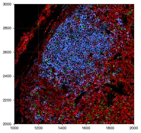
There is only one 59-channel image for each sample named origin. The default full-resolution mIF image for each slide area. Since signal intensity is very likely not to be equal between channels, we will apply an automatical linear scaling on the signals for some of the channels.
[5]:
expm.spatial_cell.image_auto_histogram(
    run_on_samples = True,
    channels = ['origin/cd4', 'origin/cd8', 'origin/dapi', 'origin/cd45', 'origin/cd20', 'origin/cd31'],
    key_added = 'adjusted',
    low_pct = 0.5,
    high_pct = 99.5
)
This added to a new image store adjusted, and copy selected channel names.
[7]:
expm.spatial_cell.summary(run_on_samples = ['a-10'])
a-10
├── origin  of shape 3727 ✗ 3726 ✗ 59
│       [ 0] dapi        [ 1] cd45        [ 2] cd11c       [ 3] bcl2        [ 4] cd90
│       [ 5] foxp3       [ 6] egfr        [ 7] p16         [ 8] pd1         [ 9] cd206
│       [10] cd45ro      [11] il10        [12] cd56        [13] cd11b       [14] cd31
│       [15] cd163       [16] cd21        [17] cd8         [18] pnad        [19] cd20
│       [20] cxcr5       [21] ki67        [22] lag3        [23] cd73        [24] cd16
│       [25] asma        [26] icos        [27] cd25        [28] coliv       [29] pdgfrb
│       [30] cd4         [31] cd68        [32] cd34        [33] vimentin    [34] podoplanin
│       [35] hladr       [36] cxcl12      [37] cd3         [38] fap         [39] cd138
│       [40] tbet        [41] periostin   [42] spp1        [43] s100a8a9    [44] clec9a
│       [45] cd45ra      [46] caix        [47] gzmb        [48] bcat        [49] sox2
│       [50] pdl1        [51] mmp9        [52] tcrgd       [53] cd38        [54] cd69
│       [55] cd15        [56] ido1        [57] mct1        [58] panck
└── adjusted  of shape 3727 ✗ 3726 ✗ 6
        [0] cd4   [1] cd8   [2] dapi  [3] cd45  [4] cd20  [5] cd31
The intensity of individual adjusted channels are quite comparable then
[11]:
fig = expm.spatial_cell.plot_spatial(
    run_on_samples = ['a-10'],
    channels = ['adjusted/cd4', 'adjusted/cd8', 'adjusted/cd20'],
    channel_colors = ['red', 'green', "#4c85ff"],
    channel_intensities = [1, 1, 1],
    plot_embeddings = { 'visible': False, },
    xrange = (1000, 2000),
    yrange = (2000, 3000),
    figsize = (5, 5),
    ticks = True
)
Integrate membrane and nuclear channel for segmentation#
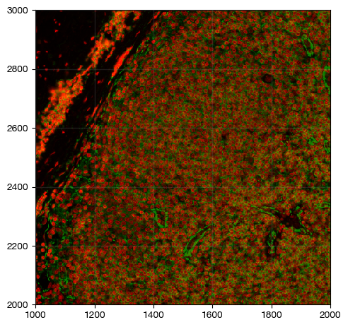
Segmentation models perform better when there are signals indicating the nucleus, cytoplasm and membrane. Since nuclear-only signal provide few information about the boundaries of cells. 10X Xenium provides a very-well demonstration for this, where they provide nuclear (Hoechst/DAPI), cytoplasma (Rps18), and boundary signals (Na/K ATPase, CD45, EPCAM) to faciliate segmentation
Here, we merge consensus membrane signal by max of each channel, and DAPI for nucleus to generate a reconstructed image for segmentation. Cytoplasmic signals are ignored.
CellPose model require an RGB image, so we will construct them in three channels. It also accepts H&E images if one consider the merged signal have less quality than an available H&E staining.
[12]:
expm.spatial_cell.image_mix_layers(
    run_on_samples = True,
    channels = ['adjusted/cd4', 'adjusted/cd45', 'adjusted/cd31'],
    mixmode = 'max',
    key_added = 'mixed-membrane',
)
[i] blended 3 channel(s) into 'mixed-membrane' for sample 'a-10'
[i] blended 3 channel(s) into 'mixed-membrane' for sample 'a-11'
image_mix_layers interface is somewhat like blend modes in Photoshop. Where multiple layers mixed to one. Yet image_mix_channels merge grayscale channels into RGB image
[18]:
expm.spatial_cell.summary(run_on_samples = ['a-10'])
a-10
├── origin  of shape 3727 ✗ 3726 ✗ 59
│       [ 0] dapi        [ 1] cd45        [ 2] cd11c       [ 3] bcl2        [ 4] cd90
│       [ 5] foxp3       [ 6] egfr        [ 7] p16         [ 8] pd1         [ 9] cd206
│       [10] cd45ro      [11] il10        [12] cd56        [13] cd11b       [14] cd31
│       [15] cd163       [16] cd21        [17] cd8         [18] pnad        [19] cd20
│       [20] cxcr5       [21] ki67        [22] lag3        [23] cd73        [24] cd16
│       [25] asma        [26] icos        [27] cd25        [28] coliv       [29] pdgfrb
│       [30] cd4         [31] cd68        [32] cd34        [33] vimentin    [34] podoplanin
│       [35] hladr       [36] cxcl12      [37] cd3         [38] fap         [39] cd138
│       [40] tbet        [41] periostin   [42] spp1        [43] s100a8a9    [44] clec9a
│       [45] cd45ra      [46] caix        [47] gzmb        [48] bcat        [49] sox2
│       [50] pdl1        [51] mmp9        [52] tcrgd       [53] cd38        [54] cd69
│       [55] cd15        [56] ido1        [57] mct1        [58] panck
├── adjusted  of shape 3727 ✗ 3726 ✗ 6
│       [0] cd4   [1] cd8   [2] dapi  [3] cd45  [4] cd20  [5] cd31
└── mixed-membrane  of shape 3727 ✗ 3726 ✗ 1
        [0] mixed
[17]:
fig = expm.spatial_cell.plot_spatial(
    run_on_samples = ['a-10'],
    channels = ['mixed-membrane/mixed', 'adjusted/dapi'],
    channel_colors = ['green', 'red'],
    channel_intensities = [1, 1],
    plot_embeddings = { 'visible': False, },
    xrange = (1000, 2000),
    yrange = (2000, 3000),
    figsize = (5, 5),
    ticks = True
)
Let’s follow the convention to place DAPI images in blue
[20]:
# this is good for segmentation
expm.spatial_cell.image_mix_channels(
    run_on_samples = True,
    channels = ['mixed-membrane/mixed', 'adjusted/dapi'],
    key_added = 'segmentation-rgb',
    channel_colors = ['green', 'blue'],
    channel_intensities = [1, 1]
)
[i] mixed 2 channel(s) into rgb written to 'segmentation-rgb' for sample 'a-10'
[i] mixed 2 channel(s) into rgb written to 'segmentation-rgb' for sample 'a-11'
[21]:
expm.spatial_cell.summary(run_on_samples = ['a-10'])
a-10
├── origin  of shape 3727 ✗ 3726 ✗ 59
│       [ 0] dapi        [ 1] cd45        [ 2] cd11c       [ 3] bcl2        [ 4] cd90
│       [ 5] foxp3       [ 6] egfr        [ 7] p16         [ 8] pd1         [ 9] cd206
│       [10] cd45ro      [11] il10        [12] cd56        [13] cd11b       [14] cd31
│       [15] cd163       [16] cd21        [17] cd8         [18] pnad        [19] cd20
│       [20] cxcr5       [21] ki67        [22] lag3        [23] cd73        [24] cd16
│       [25] asma        [26] icos        [27] cd25        [28] coliv       [29] pdgfrb
│       [30] cd4         [31] cd68        [32] cd34        [33] vimentin    [34] podoplanin
│       [35] hladr       [36] cxcl12      [37] cd3         [38] fap         [39] cd138
│       [40] tbet        [41] periostin   [42] spp1        [43] s100a8a9    [44] clec9a
│       [45] cd45ra      [46] caix        [47] gzmb        [48] bcat        [49] sox2
│       [50] pdl1        [51] mmp9        [52] tcrgd       [53] cd38        [54] cd69
│       [55] cd15        [56] ido1        [57] mct1        [58] panck
├── adjusted  of shape 3727 ✗ 3726 ✗ 6
│       [0] cd4   [1] cd8   [2] dapi  [3] cd45  [4] cd20  [5] cd31
├── mixed-membrane  of shape 3727 ✗ 3726 ✗ 1
│       [0] mixed
└── segmentation-rgb  of shape 3727 ✗ 3726 ✗ 3
        [0] r  [1] g  [2] b
Segmentation#
We currently support CellPose-SAM (v3) for segmentation, which is customizable to user’s own trainings, and provide SOTA performance and generalizability. User should configure the model initialization by themselves before passing the initialized model to exprmat. CellPose package should be installed as a dependency of exprmat.
[22]:
from cellpose.models import CellposeModel
model = CellposeModel(gpu = True)
[23]:
expm.spatial_cell.segment(
    run_on_samples = True,
    image_key = 'segmentation-rgb',
    model = model,
    mask_key_added = 'mask',
    flow_key_added = 'flow',
    batch_size = 64,
    diameter = 20,
    flow_threshold = 0.7,
    cellprob_threshold = -1
)
[i] running cellpose segmentation on 'segmentation-rgb' (3727 x 3726) for sample 'a-10'
[i] found 41491 cells
[i] running cellpose segmentation on 'segmentation-rgb' (3733 x 3732) for sample 'a-11'
[i] found 48517 cells
CellPose writes two additional layers (a mask for segmentation, and an intermediate model inference for cell boundary). See documentation of CellPose for explanations. Current masking supports only 2D images. For 3D images with sparse z-axis, It can be considered as multiple Z-level samples.
[24]:
expm.spatial_cell.summary(run_on_samples = ['a-10'])
a-10
├── origin  of shape 3727 ✗ 3726 ✗ 59
│       [ 0] dapi        [ 1] cd45        [ 2] cd11c       [ 3] bcl2        [ 4] cd90
│       [ 5] foxp3       [ 6] egfr        [ 7] p16         [ 8] pd1         [ 9] cd206
│       [10] cd45ro      [11] il10        [12] cd56        [13] cd11b       [14] cd31
│       [15] cd163       [16] cd21        [17] cd8         [18] pnad        [19] cd20
│       [20] cxcr5       [21] ki67        [22] lag3        [23] cd73        [24] cd16
│       [25] asma        [26] icos        [27] cd25        [28] coliv       [29] pdgfrb
│       [30] cd4         [31] cd68        [32] cd34        [33] vimentin    [34] podoplanin
│       [35] hladr       [36] cxcl12      [37] cd3         [38] fap         [39] cd138
│       [40] tbet        [41] periostin   [42] spp1        [43] s100a8a9    [44] clec9a
│       [45] cd45ra      [46] caix        [47] gzmb        [48] bcat        [49] sox2
│       [50] pdl1        [51] mmp9        [52] tcrgd       [53] cd38        [54] cd69
│       [55] cd15        [56] ido1        [57] mct1        [58] panck
├── adjusted  of shape 3727 ✗ 3726 ✗ 6
│       [0] cd4   [1] cd8   [2] dapi  [3] cd45  [4] cd20  [5] cd31
├── mixed-membrane  of shape 3727 ✗ 3726 ✗ 1
│       [0] mixed
├── segmentation-rgb  of shape 3727 ✗ 3726 ✗ 3
│       [0] r  [1] g  [2] b
├── mask  of shape 3727 ✗ 3726
└── flow  of shape 3727 ✗ 3726 ✗ 4
        [0] r            [1] g            [2] b            [3] probability
[25]:
fig = expm.spatial_cell.plot_spatial(
    run_on_samples = ['a-10'],
    channels = ['flow/r', 'flow/g', 'flow/b'],
    channel_colors = ['red', 'green', 'blue'],
    plot_embeddings = { 'visible': False, },
    xrange = (1500, 2000),
    yrange = (2500, 3000),
    figsize = (5, 5),
    ticks = True
)
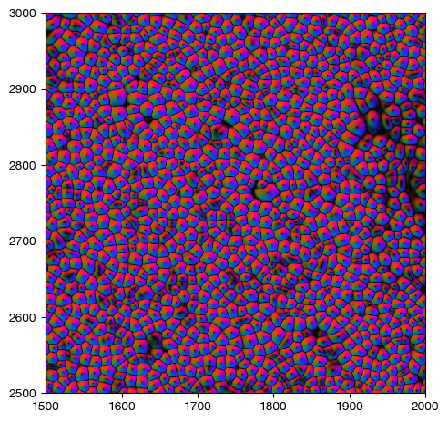
When an applicable mask is generate, segmentation is finished. For mIF images, the next step is to extract signal intensity per channel per cell to form the cell by staining matrix. For spot-based in-situ sequencing or in-situ hybridization, spots should be aggregated to form cell by feature counts. Both of them are initialization of the spatial-cell matrix
[26]:
expm.save()
[i] saving individual samples. (pass `save_samples = False` to skip)
━━━━━━━━━━━━━━━━━━━━━━━ modality [spatial-cell] 2 / 2 (00:00 < 00:00)